Vol. 59, No. 1, January 2016, pp. 35–71
TWO-SIDED MATCHING WITH EXTERNALITIES: A SURVEY
Keisuke Bando Ryo Kawasaki Shigeo Muto
Tokyo Institute of Technology
(Received September 1, 2015; Revised December 14, 2015)
Abstract The literature on two-sided matching markets with externalities has grown over the past several years, as it is now one of the primary topics of research in two-sided matching theory. A matching market with externalities is different from the classical matching market in that agents not only care about who they are matched with, but also care about whom other agents are matched to. In this survey, we start with two-sided matching markets with externalities for the one-to-one case and then focus on the many-to-one case. For many-to-one matching problems, these externalities often are present in two ways. First, the agents on the “many” side may care about who their colleagues are, that is, who else is matched to the same “one.” Second, the “one” side may care about how the others are matched.
Keywords: Game theory, two-sided matching, externalities, colleagues
1. Matching without Externalities 1.1. Introduction
Two-sided matching problems in the realm of game theory originated with the seminal paper by Gale and Shapley [25]. Their paper, in particular, looked at two problems: the “marriage” problem and the “college admissions” problem.1 In these problems, there are two distinct groups, and the objective is to form suitable pairs containing one from each group. In the case of the marriage problem, the two groups are men and women, and pairs consist of one man and one woman. Moreover, a man can be paired with at most one woman, and a woman can be paired with at most one man – hence the current name,
one-to-one matching problem. For the college admissions problem, the two sets are students
and colleges, and the objective is to form student-college pairs. In contrast to the marriage problem, while a student may be matched to at most one college, a college can be matched to more than one student, giving the problem its current name, the many-to-one matching
problem. The collection of these pairs is called a matching.
Agents on each side have what are called preferences or rankings over those on the other set; for example, students may rank colleges not just based on prestige but also based on tuition or geographic location, while colleges may rank students based on test scores, ethnicity, and other background information. When individuals have such preferences, it is not sensible to completely ignore these preferences and decide upon a matching arbitrarily. One criterion often imposed on matchings is pairwise stability or in many papers, simply called stability. To illustrate this condition, suppose that there is a man m and a woman w who want to be matched to each other instead of their respective partners. Then, m and w would find it worthwhile to dump their partners so that they elope with each other. When
1They also consider a third type of problem with pairs are to be formed from one group, which in today’s
this occurs, the original matching is dissolved, and we do not expect that matching to hold up. Roughly, a matching is said to be pairwise stable if there does not exist such a pair.
Pairwise stability is a nice concept and a relatively easy one to grasp. It is not too stringent either, as Gale and Shapley [25] not only prove the existence of a pairwise stable matching, but also provides an algorithm, called the deferred acceptance (DA) algorithm, to find one. Moreover, Roth [52] makes the observation that stability is an important factor in the success of matching mechanisms in the example of matching medical interns to hospitals. One surprising observation in that paper is that one of the mechanisms, the National Intern Matching Program (now the National Resident Matching Program), is mathematically equivalent to the DA algorithm of Gale and Shapley [25].
The theory of two-sided matching so far has many positive results. One of the key assumptions in the model is that each agent only cares about whom he/she is matched with. However, in some applications, agents may care about with whom other agents are matched. One example is envy. A student may envy another student because he/she may be matched to a prestigious school. In an economic setting, in a small industry, firms may care about who their rival firms hire. These examples all fall under matching problems with
externalities. When these externalities are present, the basic parts of the theory of standard
matching problems no longer hold. First, defining pairwise stability is not straightforward; in the example of the eloping pair, they would also need to take into account how other agents match with each other when they elope. Second, whether a pairwise stable matching exists or not depends on the particular definition of pairwise stability. In this survey, we present several lines of research that have tried to overcome these obstacles.
A model that is closely related to matching with externalities is the matching model with couples. One instance where couples have played a large role is the matching of medical interns to hospitals.2 Each intern has preferences over the different hospitals, but among the interns there may be a couple. Besides the individual preferences of each member of the couple, they would also prefer to be assigned to hospitals that are close by. In this case, one member of the couple does take into account the matching assignment of the other, so that this would be an example of a matching problem with externalities. It is also known that a stable matching may not exist (Theorem 10 of Roth [52]), and several positive results from the original matching problem do not carry over (Aldershof and Carducci [2]). Several attempts have been made to obtain positive results, such as determining a preference domain for existence (Klaus and Klijn [33]) and considering a large market (Kojima et al. [36]). We refer the reader to Bir´o and Klijn [9] for a comprehensive survey on this topic. We remark here that since the model of matching with couples treats a couple as a single agent instead of two separate agents, there are subtle differences in the stability concepts of the model with couples with those in the model with externalities. Therefore, there is not a straightforward relationship between matching with couples and the models and results presented in this survey.
Before explaining the details of these research papers, in the following, we review some essential facts in the basic theory of two-sided matching without externalities to help give the theory with externalities some context. Currently, there are many surveys and books on matching problems. To our knowledge, the list includes books by Roth and Sotomayor [59] and Gusfield and Irving [26] and surveys by Roth [56] and Roth [54] for general two-sided matching problems; Bir´o and Klijn [9] for matching problems with couples; and in relation to market design, which uses among many theories the theory of two-sided matching to
solve real-life problems involving markets, there are Roth [55] and Roth [57]. In contrast, while the literature on matching with externalities has grown recently, to our knowledge, there is no survey that provides an overall perspective on the topic. Thus, our objective in this survey is to organize some apparently disparate theories in the theory of matching with externalities.
1.2. The basic one-to-one matching model and the deferred acceptance (DA) algorithm
Let the set of agents be partitioned into two finite disjoint sets M and W , which are commonly called men and women respectively. Each m ∈ M has a strict linear ordering
≻m over W ∪ {m} where w ≻m w′ denotes that m prefers w over w′.3 This ordering ≻m is often called the strict preference relation of m.4 In addition, each w ∈ W also has an strict linear ordering ≻w over M∪ {w} indicating the preferences of w. These components together define a one-to-one (classical) matching market (M, W, (≻i)i∈M∪W).
Note that the element m is included in this list as a possibility for m to remain unmatched to any w ∈ W ; therefore, w ≻m m is interpreted as m preferring to be matched to w over being unmatched, while m≻m w is interpreted as m preferring to be unmatched over being matched to w. A woman w ∈ W is said to be acceptable to m ∈ M if w ≻m m. Likewise,
m∈ M is said to be acceptable to w ∈ W if m ≻w w.
In addition, for each i ∈ M ∪ W , denote by ⪰i the weak ordering of ≻i. For example, for m∈ M, w ⪰m w′ if w ≻m w′ or w = w′. This ordering is also used quite frequently in the literature.
A matching µ is a one-to-one mapping5 from M ∪ W to M ∪ W such that 1. µ(m)∈ W ∪ {m} for all m ∈ M,
2. µ(w)∈ M ∪ {w} for all w ∈ W , 3. µ(µ(i)) = i for all i∈ M ∪ W .
The mapping µ gives as its output the identity of the input’s partner, so that µ(m) indicates
m’s partner, and µ(w) indicates w’s partner. In order for µ to be a matching, aside from
being one-to-one, each man m’s partner must be someone in the opposite set W or m himself, while each woman w’s partner must be someone in the opposite set M or w herself. The first two conditions state this property formally. Moreover, if w is m’s partner, then m must be w’s partner, which is the third condition. The objective in this matching market is to find a matching µ that satisfies some suitable property.
A matching µ is said to be pairwise stable if it satisfies the following two conditions:
• For each i ∈ M ∪ W , µ(i) ⪰i i.
• There does not exist a pair (m, w) ∈ M × W with µ(m) ̸= w such that m ≻w µ(w) and
w≻m µ(m).
The first condition is often called individual rationality. If i ≻i µ(i), then i would prefer to be single, and because each agent has an option to be single, individual rationality is a minimal requirement for a matching to persist. The second condition states that no pair would find it worthwhile to dump their partners under µ to be matched to each other. Such a pair is typically called a blocking pair with respect to µ. If there is such a blocking pair, then the matching µ will likely be dissolved. Roth [52] finds that in the matching market of
3A linear ordering is such that every element is comparable, and that the ordering satisfies transitivity. 4The term “strict” is used to denote that given two different women w and w′ in W , m can either rank one
strictly lower or higher than the other. In other words, m is not faced with a situation involving two women that he equally likes. This same restriction is also imposed on the preferences of w.
medical interns to hospitals, this stability property distinguishes those matching processes that last from those that are abandoned.
Note that any stable matching µ is Pareto efficient; that is, there is no matching ν such that ν(i) ⪰i µ(i) for all i ∈ M ∪ W and ν(j) ≻j µ(j) for some j ∈ M ∪ W . To see this, suppose otherwise. Without loss of generality, we assume that ν(m) ≻m µ(m) for some
m ∈ M. By individual rationality of µ, we have that ν(m) ∈ W , which we denote by w.
Then, we have that m ⪰w µ(w). By ν(m) ̸= µ(m), we have that ν(w) ̸= µ(w), which implies m≻w µ(w) because ≻w is strict. This contradicts that µ is stable.
While pairwise stability seems to be a rather strong property, Gale and Shapley [25] show that for any matching market, there exists at least one pairwise stable matching. Moreover, they define an algorithm, called the deferred acceptance (DA) algorithm, that produces a pairwise stable matching. Below is a verbal description of the algorithm.
(Men-proposing) DA Algorithm (One-to-one Case)
(Step 1.a) Each man m ∈ M proposes to w ∈ W whom he likes the most among those acceptable to m. If no such w ∈ W exists, m is matched to himself.
(Step 1.b) Each woman w ∈ W chooses the most preferred m ∈ M who proposed to
w and rejects all other men who have proposed to her. In such a case, m and w are
tentatively matched to each other.
· · ·
(Step k.a) Each man m∈ M proposes to w ∈ W whom he likes the most among those acceptable to m and who has not rejected m at an earlier step. If no such w ∈ W exists,
m is matched to himself.
(Step k.b) Each woman w ∈ W chooses the most preferred m ∈ M who proposed to
w and her tentative partner and rejects all other men. In such a case, m and w are
tentatively matched to each other.
The algorithm ends when no man m∈ M is rejected, and the tentative matching becomes the final matching. Gale and Shapley [25] show that this procedure yields a stable matching. To understand the basic reasoning, consider m ∈ M, and let µM be the matching that is produced from the above DA algorithm.
To disrupt the stability of the matching, m needs to find a w with w ≻m µM(m) and m ≻w µM(w). When running this algorithm, m must have proposed to w at some point since w is ranked higher than µM(m). Because m is not ultimately matched to w, w must have rejected m at some point. The reason why w would reject m is that w rejected m’s proposal to accept someone whom she prefers over m or she accepts m’s proposal but accepts a proposal from a different man m′ in favor of m. Because each woman in the procedure always accepts a proposal from someone whom she likes more, w’s ultimate partner must be preferred over m by w.
The key argument is that when w rejects m, w never regrets letting m go, as once w rejects m, w is always tentatively matched to a man that she prefers over m. This is a result not just from the algorithm itself, but on the basic assumption of the preferences. In more complex models, more assumptions on preferences are made so that this “regret-free” property still holds. It should be noted here that with preferences of w of m over m′ that are dependent on whom her rival, say w′ is matched to, the previous argument may not hold, thereby implying some of the complexity behind matching problems with externalities. We will come back to this issue in Section 2.
is best matching among pairwise stable matchings for the agents in M . Such a matching is said to be M -optimal.
Theorem 1.1 (Gale and Shapley [25]). Let µM be the matching that is produced from the above DA algorithm with men-proposing and let µ be any pairwise stable matching. Then, µM is pairwise stable and µM(m)⪰
m µ(m) for all m∈ M.
A DA algorithm can also be defined with the roles of M and W reversed so that women propose to men. Then, the matching that results is pairwise stable and W -optimal. More-over, it is shown that the W -optimal stable matching is M -worst in that all members in
M are weakly worse off compared to any other pairwise stable matching. Similarly, the M -optimal matching µM is also W -worst.
The model outlined so far imposes the restriction of each m being matched to one w (or unmatched). However, in examples such as matching interns to hospitals or students to schools, the hospitals or schools often admit more than one intern or student. In the next section, we explain the extension of the model to fit these applications.
1.3. Extension to many-to-one matching markets
In this section, we outline the basic model of matching markets where one side can be matched to more than one agent on the other side. However, we maintain the restriction on the other side so that one student can only be admitted to at most one school. This model corresponds to the “college admissions” model in Gale and Shapley [25].
Instead of M and W being the two disjoint sets, in this model, we consider a matching market with disjoint sets S and C, where an element in S is called a student, and an element in C is called a college or school.6 Each student can be matched to at most one school, while a school may admit more than one student.
As before, each s∈ S has a strict preference ordering over C ∪ {∅}, labeled by ≻s, where ∅ denotes that s is not matched to a c ∈ C. Each college c ∈ C has strict preferences ≻c over 2S := {S′|S′ ⊆ S}. Given a set S′ ⊆ S, denote by Ch
c(S′), called the choice set, the top group of students in S′ for c. That is, Chc(S′) denotes the set T ⊆ S′ such that T ⪰c S′′, ∀S′′ ⊆ S′. Because preferences are more general, choice sets give us a compact way of defining analogues to the concepts discussed in the previous simpler models.
A matching is a set-valued mapping µ from C ∪ S to itself, satisfying the following conditions.
1. For each s∈ S, either µ(s) = {c} for some c ∈ C or µ(s) = ∅. 2. For each c∈ C, µ(c) ⊆ S
3. For s∈ S and c ∈ C, µ(s) = {c} if and only if s ∈ µ(c).
A matching is said to be individually rational if for each s∈ S, µ(s) ⪰s ∅ and for each
c ∈ C, µ(c) = Chc(µ(c)). The main difference is the condition for c ∈ C. Because each
c ∈ C can unilaterally reject students in µ(c), if µ(c) ̸= Chc(µ(c)), then Chc(µ(c)) ⊊ µ(c) and Chc(µ(c)) ≻cµ(c), so that college c would benefit from rejecting those in µ(c) but not in Chc(µ(c)).
A matching is pairwise stable if there does not exist a pair (c, s) ∈ C × S with s /∈ µ(c) such that c ≻s µ(s) and s ∈ Chc(µ(c)∪ {s}). If such a pair were to exist, then with s preferring c to his/her assigned college µ(s), c would also prefer to admit s, possibly with the cost of rejecting some students in µ(c).
6While the notation for one-to-one matching problems is usually M and W or M and F (for female), the
notation for the many-to-one model may differ depending on the context. In this survey, for the models discussed, we mostly adhere to the notation used in the original papers.
We introduce an assumption called substitutability that is widely used in the literature. Preferences ≻c is said to satisfy substituability if for all T ⊆ S and s, s′ ∈ T with s ̸= s′,
s∈ Chc(T ) ⇒ s ∈ Chc(T \ {s′}).
Substitutability essentially eliminates any complementarities between any two students s and s′. The unavailability of s′ should not affect the desirability of college c’s to include s. The condition in its form for two-sided matching problems originates from Roth [53] and is an adaptation of the gross substitutes condition defined in Kelso and Crawford [31]. These substitutability conditions have also been connected to the literature on discrete convexity. Fujishige and Yang [24] first connects gross substitutability of Kelso and Crawford [31] to M♮-convexity of Murota and Shioura [45], which is an equivalent variant of Murota [43, 44]. Subsequent matching models that have used discrete convexity include (and are not confined to) Danilov et al. [13], Fujishige and Tamura [23], Murota and Yokoi [46], and Kojima et al. [37]. For a comprehensive survey on this direction, we refer the reader to the survey by Shioura and Tamura [63].
A more useful equivalent expression of substitutability is given by
s /∈ Chc(T \ {s′}) ⇒ s /∈ Chc(T ).
Repeated application of the above expression yields the following. Let T ⊆ T′ ⊆ S. Then,
s /∈ Chc(T )⇒ s /∈ Chc(T′).
The above form is the one given in the literature of matching with contracts in Hatfield and Milgrom [28].
Substitutability ensures that a pairwise stable matching exists. A modification of the DA algorithm can be used to show this fact.
(Student-proposing) DA Algorithm (Many-to-one Case)
(Step 1.a) Each s∈ S applies to the top-ranked college c ∈ C according to ≻s.
(Step 1.b) For each c ∈ C, let A1c be the set of students that apply to c. Then, c ∈ C tentatively keeps Chc(A1c) and rejects the rest. For notational ease, let Tc1 := Chc(A1c) be the set of students that are kept by c.
· · ·
(Step k.a) Each s ∈ S applies to the top-ranked college c ∈ C among those that have not rejected s.
(Step k.b) Let Ak
c be the set of students that newly apply to c ∈ C. Each c ∈ C tentatively keeps Chc(Akc∪ Tck−1) where Tck−1 is the set of students that c ∈ C kept after Step k− 1.b, and rejects the rest.
The algorithm ends when no students are rejected. This version of the DA algorithm also yields a pairwise stable matching. The argument behind this result is the same as in the one-to-one case. Each college when rejecting a student does not regret doing so. This fact is reflected in the substitutability assumption.
To illustrate the logic, suppose that s is rejected in Step 1.b, thereby implying that
s /∈ Chc(A1c) = Tc1. Note that Chc(Tc1∪{s}) = Chc(Tc1) = Tc1, since Tc1 is the most preferred set when A1
c is the set of available students, then it must also be the most preferred when Tc1∪ {s} is the set of available students.7 Therefore, s /∈ Chc(Tc1) must also hold. In the 7The first equality is a direct consequence of a property of choice sets called consistency, while the second
next period, the set of students A2
c additionally apply to c, and c is faced with choosing a subset from Tc1 ∪ A2c. Consider the hypothetical situation in which s is available so that the set of alternatives is T1
c ∪ A2c ∪ {s}. Then, by substitutability, s /∈ Chc(Tc1∪ {s} ∪ A2c). Therefore, once s is rejected, there is no scenario in which c would want to add s in the subsequent steps.
Another line of research to establish existence along with the lattice structure of pair-wise stable matchings is to use Tarski’s fixed point theorem. This line of research has its origins in Adachi [1] for one-to-one matching markets and has been used extensively in more complex models, including those that are covered extensively in this survey. We relegate the discussion on this topic until Section 3.
1.4. Summary and overview of the contents of this survey
Thus far, we have provided an overview on the results of two-sided matching markets without externalities in the one-to-one case and in the many-to-one case. This is only a sliver of the numerous results in the literature, and for the interested reader on this topic, we refer the reader to some of the literature listed in at the end of Section 1.1.
An underlying assumption in these models made on the preferences of each individual, was that each m∈ M, for example, had preferences over W that were independent of how other people were matched. As stated in the introduction, envious agents are examples in which preferences may be dependent on the matching. In Section 2, we first outline the results on the literature for one-to-one matching markets with externalities. These situations arise, for example, in collegiate sports in which these colleges compete with each other through sports leagues. These examples can also be extended to matching problems between firms and workers, sports teams and athletes, or research facilities and researchers. It should be noted that the regret-free property that made the DA algorithm work does not hold in the model with externalities. Because preferences can be contingent on the matching of other agents, w may reject m at some point, but would want m back at a later point when the matchings of other agents have changed.
The asymmetry in the many-to-one case introduces a categorization of externalities that can only appear in many-to-one matching problems. One example of such externality is the many-to-one matching problem with colleagues. In terms of the student-school example, a student not only cares about the school to which he/she is matched, but also takes into account the other students matched to the same school – that is, his/her colleagues. Schools are assumed to only care about which set of students to admit and does not care about how others schools are matched. This specific form of externality does not appear in the one-to-one model since there were no “other students” that were matched to the same school. However, if we decompose the slots of each school into individual agents and view this problem as an artificial one-to-one matching problems, this would be a case of a matching problem with externalities without any specific label. We review the literature on this model in Sections 3 and 4.
2. Basic Models of Matching with Externalities
In this section, we introduce a matching problem with externalities, in which each agent cares not only his/her match but also on the matching of the other agents. When such externalities exist, it is not straightforward to define a stability concept because a stability of a matching depends on how a deviating pair expects the reaction of the other agents. Since Sasaki and Toda [61, 62] initiates the study on the matching problem with externalities, various stability concepts are proposed and these properties are investigated. We summarize
the studies on matching problems with externalities. We also briefly summarize the recent development on the literature.
2.1. The one-to-one model and stability concepts
Sasaki and Toda [62], along with its working paper version Sasaki and Toda [61], are to our knowledge the earliest papers that consider matching with externalities for one-to-one matching problems. In their papers, they define several stability concepts for this model.
Let M and W be disjoint finite sets. Recall that in the matching model without ex-ternalities, a matching µ is pairwise stable if there does not exist a pair (m, w) ∈ M × W such that m ≻w µ(w) and w ≻m µ(m). The implicit assumption is that m and w can together leave their respective partners and be matched with each other. Whether such a move benefits both m and w did not matter how the other agents were matched. It may be the case that m may prefer to be matched with w if his former partner µ(m) remained unmatched, but may find it loathsome if µ(m) were matched to his nemesis, say m′. This is just one example of a case in which there are externalities; other examples include matchings between professional sports athletes and teams and matchings between workers and firms that compete with each other.
To incorporate this possibility, for each m ∈ M, instead of ≻m being a preference ordering over W ∪ {m}, now ≻m is a preference ordering over the set of all matchings, denoted M. Similarly, for w ∈ W , ≻w is a preference ordering over M as well. Assume that all preferences are strict so that for each i∈ M ∪ W and for all µ ̸= µ′, either µ≺i µ′ or µ≻i µ′.
One complicating issue for matching with externalities involves deciding on a stability concept. In principle, the idea should be the same; a matching µ should be deemed unstable if there exists a pair (m, w), not matched with each other in µ, but would benefit from being matched with each other than with their partners µ(m) and µ(w) respectively. However, whether such a defection from µ is beneficial depends heavily on how the others are matched. Mathematically, for a pair (m, w) define M(m, w), the set of matchings in which m and w are matched, by
M(m, w) = {µ ∈ M|µ(m) = w}.
It could be the case that for some µ′ ∈ M(m, w), µ′ ≻m µ and µ′ ≻w µ, while for some µ′′ ∈ M(m, w), it may be the case that µ′′ ≺m µ. Also, there is a matching ¯µ∈ M(m, w) such that ¯µ is the matching induced by the deviation of (m, w) that keeps all other agents’
assignments “unchanged, if possible.” To express the phrase in quotation marks formally, we say that ¯µ is induced from µ by the pair (m, w) if the following conditions are satisfied:
• ¯µ ∈ M(m, w),
• ¯µ(i) = µ(i) for all i /∈ {m, w, µ(m), µ(w)}, • ¯µ(j) = j for j ∈ {µ(m), µ(w)}.
We use the notation µ→m,wµ if ¯¯ µ satisfies the conditions above.8 Note that ¯µ is a particular matching inM(m, w) and so represents a particular expectation held by both m and w over
M(m, w).
Sasaki and Toda [61] define three types of stability concepts based on the expectations of m and w over the matchings in M(m, w). Let µ ∈ M and let m and w be such that
8The notation is borrowed from Chwe [11], who calls it an effectiveness relation, and is used prominently in
the literature that considers farsighted agents – agents who can anticipate sequences of deviations and are only interested in the final outcome of those deviations. See Mauleon et al. [41] and Klaus et al. [34] for the use of this notation in matching markets. In contrast, agents in this survey are myopic – they only consider the immediate consequence of their deviations.
µ(m)̸= w.
1. m and w optimistically blocks µ if for some µ′ ∈ M(m, w), µ′ ≻m µ and µ′ ≻w µ. 2. m and w conservatively blocks µ if for all µ′ ∈ M(m, w), µ′ ≻m µ and µ′ ≻w µ. 3. m and w blocks µ if for the matching ¯µ such that µ→m,w µ, ¯¯ µ≻m µ and ¯µ≻w µ.
In the first definition, the pair (m, w) deviates from µ if in the best scenario, m and w are better off by doing so. This optimism is reflected in the condition “for some µ′ ∈ M(m, w).” In the second definition, the pair (m, w) deviates from µ if even in the worst scenario, m and w are better off by doing so. This conservatism is reflected in the condition “for all
µ′ ∈ M(m, w).” In the third definition, the matching ¯µ reflects the matching in which m
and w are matched with each other, those who were previously matched with m or w (µ(m) and µ(w)) are single (that is, matched with himself or herself), and all others uninvolved remain matched to the same partners under ¯µ.9
Recalling from the definition of stability in the case when there are no externalities, we also need to define concepts of individual rationality. To do so, we define an analogue
of M(m, w) involving the set of matchings that result when an agent i breaks up with a
partner to be alone. For i∈ M ∪ W , define
M(i) = {µ ∈ M|µ(i) = i}.
That is,M(i) represents all matchings in which i is single.
Then, we can also define a matching ¯µ to be induced from µ via a single agent i ∈ M ∪W ,
denoted by µ→i µ if the following conditions are satisfied.¯ • ¯µ ∈ M(i),
• ¯µ(j) = j for j = µ(i),
• ¯µ(k) = µ(k) for all k ̸= i, k ̸= µ(i).
Similarly, we can define three types of individual rationality conditions, which correspond to the different expectations that an agent i ∈ M ∪ W have over possible matchings that may result from i being single.
1. A matching µ is optimistically individually rational (O-IR) if there do not exist i ∈
M ∪ W and a matching µ′ ∈ M(i) such that µ′ ≻i µ.
2. A matching µ is conservatively individually rational (C-IR) if there does not exist i ∈
M ∪ W such that for all µ′ with µ∈ M(i), µ′ ≻i µ.
3. A matching µ is individually rational (IR) if there does not exist i∈ M ∪ W such that for the matching µ′ such that µ →i µ′, µ′ ≻i µ.
The stability of a matching can be defined using each of the three definitions of blocking and their corresponding individual rationality conditions. The three different definitions of stability are given in the following. Let µ∈ M.
1. µ is optimistically stable (O-stable) if it is O-IR and there do not exist a pair (m, w) with µ(m)̸= w such that (m, w) optimistically blocks µ.
2. µ is conservatively stable (C-stable) if it is C-IR and there do exist pair (m, w) with
µ(m)̸= w such that (m, w) conservatively blocks µ.
3. µ is pairwise stable (P -stable) if it is IR and there do not exist pair (m, w) with µ(m)̸= w such that (m, w) blocks µ.10
9In most papers, when a pair (m, w) deviates, the matching ¯µ is the one that results. Details about how
agents other than m and w are matched were not needed in defining stability concepts for matching without externalities. ¯µ is the matching with the minimum number of changes to have m and w be matched to each
other.
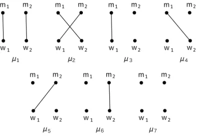
m1 m2 w1 w2 m1 m2 w1 w2 m1 m2 w1 w2 m1 m2 w1 w2 m1 m2 w1 w2 m1 m2 w1 w2 m1 m2 w1 w2 μ1 μ2 μ3 μ4 μ5 μ6 μ7
Figure 2.1: 7 matchings in Example 2.1
Now, let us introduce the following notation:
• SO: the set of O-stable matchings • SC: the set of C-stable matchings • SP: the set of P -stable matchings
With externalities, three stability concepts are different (See Example 2.1). Therefore, a stability of a matching depends on how a deviating pair or a single agent anticipates the reaction of the other agents.
Sasaki and Toda [61] shows the following results.
Theorem 2.1 (Sasaki and Toda [61]). Let SO, SC, and SP be defined as above. Then, the following statements hold.
1. SO ⊆ SP ⊆ SC and SC ̸= ∅.
2. Every matching µ ∈ SO is Pareto efficient. That is, there is no µ′ ∈ M such that for
µ′ ⪰i µ for all i∈ M ∪ W and µ′ ≻j µ for some j ∈ M ∪ W . 3. There exists at least one matching µ∈ SC that is Pareto efficient.
Theorem 2.1 highlights some strengths and weaknesses of SC and SO. SC has the advantage that it is always nonempty, but not every C-stable matching is necessarily Pareto efficient. The following example illustrates this fact. This example also illustrates that
SO ⊊ SP ⊊ SC.
Example 2.1. Let M ={m1, m2} and W = {w1, w2}. There are 7 matchings in this market which are denoted by Figure 2.1. m1’s preferences are given by:
≻m1: µ2, µ5, µ7, µ1, µ6, µ3, µ4.
This means that m1 ranks µ2 first, µ5 second, and so on. We assume that there are no externalities on m2 in that there exists an ordering ≻∗m2 over W ∪ {m2} such that for all w, w′ ∈ W ∪ {m2}, w ≻∗m2 w
′ if and only if µ ≻
m2 µ′ for all µ ∈ M(m2, w) and all µ′ ∈ M(m2, w′). In this case, we can focus only on the associated ordering to check the blocking conditions and IR conditions. Specifically, m2’s preferences and the associated the abbreviation P -stable for “pairwise stable.” We have chosen the names here to avoid confusion in the abbreviation of the terms.
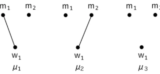
μ1 μ2 μ3 m1 m2 w1 m1 m2 w1 m1 m2 w1
Figure 2.2: 3 matchings in Example 2.2 ordering are given by:
≻m2: µ2, µ5, µ1, µ6, µ3, µ4, µ7 (≻
∗
m2: w1, w2, m2).
Similarly, we impose the same conditions on the women as on m2. Their preferences and the associated orderings are given by:
≻w1: µ1, µ3, µ2, µ5, µ6, µ4, µ7 (≻ ∗ w1: m1, m2, w1) ≻w2: µ1, µ6, µ2, µ4, µ5, µ3, µ7 (≻ ∗ w2: m2, m1, w2).
In this market, we can show that SO ⊊ SP ⊊ SC. To see this, we first consider µ2. It is easy to see that µ2 is O-IR. Moreover, each man ranks µ2 first. This implies that µ2 is
O-stable.
Next, consider µ1. Then, it is O-IR for m2, w1 and w2. For m1, µ1 is IR, but not
O-IR because µ7 ≻m1 µ1 ≻m1 µ6 holds. Moreover, µ1 is ranked first for each woman, which
implies that µ1 is P -stable, but not O-stable.
Next, consider µ5. This matching is IR. However, it is blocked by (m1, w2) and hence is not P -stable. On the other hand, the same pair cannot C-block µ5 because m1 anticipates that µ4 occurs when he deviates with w2 under the pessimistic expectation. Moreover, µ5 is not C-blocked by (m2, w2) and (m1, w1). Therefore, µ2 is C-stable, but not P -stable.
Note that µ3, µ4, and µ7 are not C-stable because these are C-blocked by an unmatched pair. Moreover, µ6 is not C-stable because it is C-blocked by (m2, w1).
From the above arguments, in this example, we have that
SO ={µ2}, SP ={µ1, µ2}, SC ={µ1, µ2, µ5}.
In this market, C-stability does not imply Pareto efficiency. In fact, all agents strictly
prefer µ2 to µ5, and hence µ5 is not Pareto efficient. □
All matchings in SO are at least Pareto efficient, but such matchings are not guaranteed to exist. Therefore, key properties of existence and efficiency that held for pairwise stable matchings for the case without externalities do not hold for each of the stable matchings considered thus far. The following example illustrates that SO and SP are empty.
Example 2.2. Let M = {m1, m2} and W = {w1}. In this market, there are 3 matchings which are denoted by Figure 2.2. Each agent’s preferences are given by:
≻m1: µ3, µ1, µ2 ≻m2: µ2, µ1, µ3 ≻m3: µ1, µ2, µ3
First, µ1 is not IR because µ3 ≻m1 µ1 holds. Next, µ3 is blocked by (m2, w1) and the
resulting matching is µ2. However, µ2 is blocked by (m1, w1). Therefore, SP and SC are
It should be noted that the DA algorithm cannot be used directly in the current setting. For m∈ M, it may not be clear who in w ∈ W is ranked the highest in m’s list as m also may take into account how other agents are matched. This dependence also disrupts one of the key properties of the success of the DA algorithm. When w ∈ W rejects m ∈ M, w does not regret doing so as she can hold on to a more favorable man, say m′. However, w’s preference of m′over m may be reversed based on how other agents are matched throughout the process. In Section 2.3.3, we will give a formal discussion on the failure of the DA algorithm.
The nonemptiness of a C-stable matching, nonetheless, can be proved by artificially constructing a two-sided matching problem without externalities. Consider m ∈ M and
w, w′ ∈ W . Let µ ∈ M(m, w) be the least-preferred matching for m in the set M(m, w) –
that is, µ ⪯m µ for all ˜˜ µ ∈ M(m, w). Similarly, let µ′ ∈ M(m, w′) be the least-preferred matching for m in the set M(m, w′). Define the relation≻∗m by
w≻∗m w′ ⇔ µ ≻m µ′.
Repeat for all pairs in W ∪ {m} to obtain binary comparisons of ≻∗m. Because the original preferences ≻m satisfies transitivity,≻∗m should yield a linear ranking over W∪{m}. Define a similar preference relation ≻∗w for each w ∈ W over M ∪ {w}. Then, (M, W, (≻∗i)i∈M∪W) defines a two-sided matching market without externalities. Using the DA algorithm, there exists a pairwise stable matching µ∗ in (M, W, (≻i)i∈M∪W), which is also a C-stable matching in the original market (M, W, (≻i)i∈M∪W) with externalities.
The following example illustrates the above construction. This example also illustrates that, in the associated one-to-one matching market (M, W, (≻∗i)i∈M∪W), while we can find at least one C-stable matching, we cannot find a Pareto efficient C-stable matching.
Example 2.3. Consider the same market as in Example 2.1. The associated one-to-one
matching market without externalities is given by:
≻∗ m1: m1, w1, w2 ≻ ∗ m2: w1, w2, m2 ≻ ∗ w1: m1, m2, w1 ≻ ∗ w2: m2, m1, w2.
In this market, the unique stable matching is given by µ5. However, the set of stable matchings in the associated market includes only the Pareto inefficient C-stable matching. Therefore, we cannot find a Pareto efficient C-stable matching unless focus on the original
market. □
Example 2.3 shows that the associated one-to-one matching market may miss a Pareto efficient C-stable matching. Nevertheless, Theorem 2.1 states that there exists at least one Pareto efficient stable matching. To obtain this result, the key property is that if a C-stable matching µ is Pareto dominated by another matching ν, then ν is also C-C-stable. By repeatedly using this property, we can show the existence of a Pareto efficient C-stable matching.
While the focus has been on SO and SC, much of the recent literature focuses on SP and variants of it due to the ease of interpretation of this stability concept. It is much in the spirit of Nash equilibrium in that when agents deviate, they assume that the situation involving other agents has not changed. However, Theorem 2.1 is silent about the existence of a
P -stable matching. Mumcu and Saglam [42] derives a sufficient condition for the existence
of a P -stable matching, based on a condition, called the top-coalition property, that is used for the existence of a core coalition structure for hedonic games introduced in Banerjee et al. [8].
Formally, let Pi[k] be the kth best matching according to i’s preferences. A set of matchings V is a top matching collection if V ̸= ∅ and for each µ ∈ V and for each i, there exists k≤ |V| such that µ = Pi[k].
Informally, the top matchings collection is the set of matching consisting of k matchings such that each individual i ∈ M ∪ W can all agree to the fact that “the top k matches in terms of preferences are included in this set.” Conversely, every individual would consider each matching outside this set to be ranked number k + 1 or below.
We now present the result of Mumcu and Saglam [42], rewritten in terms of the language introduced in this survey.
Theorem 2.2 (Mumcu and Saglam [42]). If a top matching collection V satisfies the
fol-lowing condition (*), then V ⊆ SP, and so SP ̸= ∅.
(*) For all µ, µ′ ∈ V, either one of the following conditions hold: (i) if there exists a pair µ, µ′ ∈ V such that µ →m,w µ′ for some (m, w), then either µ′ ≺m µ or µ′ ≺w µ; (ii) µ→i,j µ′ does not hold for any (i, j) ∈ M × W or i = j (this condition summarizes (ii) and (iii) of the original statement).
The conditions in Theorem 2.2 eliminate the cases in which one of the matchings in
V acts as the matching ¯µ towards another matching also in V, thereby making the latter
matching not P -stable. Essentially, what the theorem states is that to check P-stability, first consider the matchings in V and then to check whether blocking can occur within just the set V itself.
Subsequent papers that extend analysis of matching with externalities to broader ing problems, such as many-to-one matching problems, focus primarily on P -stable match-ings. These extensions will be summarized later in this survey. In what follows, we return to the paper of Sasaki and Toda [62], which define estimation functions, as one of the extensions that keep the one-to-one structure intact.
2.2. An extension of the one-to-one model using estimation functions
In the definitions of the stability concepts, it was assumed that when m and w consider deviating from a matching µ, they considered all or some of the possibilities from the set
M(m, w). Instead, they may assume that some of those matchings in M(m, w) are not
sensible for whatever reason. Sasaki and Toda [62] use what is called an estimation function to describe the set of matchings that m and w each thinks is plausible among those in
M(m, w). In Sasaki and Toda [62], these estimations are defined a priori and are defined
independently of the preferences of agents.
For expositional ease, consider the case when there is an equal number of men and women, and the set of feasible matchings are those in which each man m is matched to a woman w and vice-versa. Thus, there is no agent that is not matched.
Formally, let m ∈ M and denote by φm(w) the set of matchings µ that m perceives will occur if matched to w. Since m considers the possibilities of matchings that involve
m matched with w, φm(w) ⊆ M(m, w) for all w ∈ W . This function φm defined on W
constitutes the estimation function of m ∈ M. Similarly, for w ∈ W , we can define an estimation function φw.
Using the estimation functions, we can extend the definition of stability of matchings to this setting. Sasaki and Toda [62] only considers C-stable matchings for this setting, as one of the objectives is to investigate the extension of the existence result (Theorem 2.1).
Let estimation functions φi be defined for all i ∈ M ∪ W . A matching µ is said to be φ-stable if there does not exist a pair (m, w) such that
µ′ ≻m µ, ∀µ′ ∈ φm(w) and
That is, when considering the stability of a matching µ, m looks at all matchings that
m expects to occur when matched to w, which is denoted by φm(w), and w looks at all
matchings that w expects to occur when matched to m, which is denoted by φw(m). Note that it need not be the case that φm(w) = φw(m) so that m and w need not agree on the estimation of the matchings that could be realized when matched to each other.
Sasaki and Toda [62] show a rather negative result regarding the existence of φ-stable matchings. Unless φm(w) = φw(m) = M(m, w), there exists an instance which does not admit a φ-stable matching. This result is a sharp contrast to the existence result stated earlier in Theorem 2.1. The formal statement is as follows.
Theorem 2.3 (Sasaki and Toda [62]). Let M and W be two disjoint sets. Suppose that
for some m ∈ M and w ∈ W , φm(w)̸= M(m, w). Then, there exists a preference profile
(≻i)i∈M∪W such that the matching market (M, W, (≻i)i∈M∪W) does not admit a φ-stable matching.
This negativity result is based on the fact that φ is fixed at the very beginning. In an extreme setting, these estimation functions can be arbitrary because they are defined independently from the preferences of the agents. As a modification to these estimation functions, Li [40] defines what are called rational expectations to make these estimation functions consistent.11 When m and w deviate to form a pair, they should expect the set of agents M\ {m} and W \ {w} to be matched in a “stable” way. The formal definition starts with the usual definition of pairwise stability for a market with two agents each. Then, the definition proceeds for markets with more agents through a recursive formulation.
Hafalir [27] takes a different approach centered around the negativity result of Theorem 2.3. The trick behind the negativity result of Theorem 2.3 is that for a given profile of estimation functions for each i ∈ M ∪ W , we can construct preferences such that φ-stable matchings do not exist without arguing whether estimations were sound based on the pref-erences at hand. Hafalir [27] first limits the estimation functions that can be construed based on the preferences of the agents. In this sense, estimation functions are endogenously given. Hafalir [27] then defines what are called sophisticated estimation functions and shows that these estimation functions can circumvent the negative result of Sasaki and Toda [62]. These estimation functions, like those of Li [40], are defined inductively. We refer the reader to the original paper for details.
2.3. Many-to-one matching markets with externalities among firms
In this section, we analyze the model of many-to-one matching with externalities among firms. That is, each firm’s preferences depend not only on its workers, but also on the matching of its rival firms. Externalities do not exist among workers. This model is an extension of the model of Sasaki and Toda [61, 62] into a many-to-one matching market. In fact, we can directly apply the approach of Sasaki and Toda [61, 62] into this model. Bando [6, 7] takes a different approach from Sasaki and Toda [61, 62]. As we saw in Section 1.3, the choice function is a useful tool to analyze a classical model. Bando [6, 7] extends the choice function approach into the market with externalities. We summarize the results of Bando [6, 7].
2.3.1. Model
Let F ={f1, . . . , fm} be the set of m firms and W = {w1, . . . , wn} be the set of n workers. Each firm can hire multiple workers, but each worker is allowed to work at most one firm. A matching µ is a function from F ∪ W into 2F∪W such that (i) for each w ∈ W , either
11Technically, Li [40] is not a paper on matching theory but on principal-agent problems, which is closely
µ(w) = {f} for some f ∈ F or µ(w) = ∅, (ii) for each f ∈ F , µ(f) ⊆ W , and (iii) for each
w∈ W and f ∈ F , µ(w) = {f} if and only if w ∈ µ(f). Let M be the set of matchings. We
often regard a matching µ as a tuple (µ(f1), . . . , µ(fm)). For µ∈ M, f ∈ F and C ⊆ W , define a matching µf,C as follows:
if w∈ C, then µf,C(w) ={f}, if w ∈ µ(f) \ C, then µf,C(w) = ∅, if w /∈ C ∪ µ(f), then µf,C(w) = µ(w).
In other words, µf,C is a matching that is obtained from µ by satisfying f and C, keeping the matching of the other agents fixed. For µ∈ M and f ∈ F , we write ∪f′∈F \{f}µ(f′) by µ(−f). That is, µ(−f) is the set of workers who are hired by f’s rival firms in µ.
Each firm f has a strict preference ordering ≻f over the set of matchings M. Each worker w has a strict preference ordering ≻w over F ∪ {∅}, where “∅” represents being unmatched. We say that f is acceptable for w when f ≻w ∅.
We next define choice functions for firms. In a classical model, for any subset of workers
C, firm f ’s choice function Chf(C) is f ’s most preferred workers among C. In our model, f ’s choice function may depend on the matching of the other firms. To define a choice
function, we need to introduce additional notations. For f ∈ F and C ⊆ W , define
R(f, C) ={µ ∈ M|µ(f) = ∅ and µ(w) = ∅ for all w ∈ C},
which is the set of matchings such that all workers in C are unemployed and firm f does not hire any workers. Then, f ’s choice function Chf(C|µ) is defined as firm f’s most preferred subset of C given µ ∈ R(f, C). That is, Chf(C|µ) is the set such that (i) Chf(C|µ) ⊆ C and (ii) µf,Chf(C|µ) ⪰
f µf,C
′
for all C′ ⊆ C.
Throughout, we assume that each firm’s choice function depends on µ only through the workers hired by rival firms.12 That is, for any f ∈ F , any C ⊆ W and any µ, µ′ ∈ R(f, C),
µ(−f) = µ′(−f) implies Chf(C|µ) = Chf(C|µ′). Under this assumption, we can regard a choice function as a function from△ to 2W, where
△ := {(C1, C2)|C1, C2 ⊆ W with C1∩ C2 =∅}.
We next define the stability concept provided by Bando [6]. As we saw in Section 2.1, when externalities exist, the stability of a matching depends on how a deviating pair expects the reaction of the other agents. We assume that a firm and workers deviate from a matching, assuming that the matching of the other agents is unchanged. This is the same assumption as that behind the P -stability provided in Section 2.1.
We first recall the definition of P -stable matching. A matching µ is individually rational if µ(w) ⪰w ∅ for all w ∈ W and Chf(µ(f ))|µ(−f)) = µ(f) for all f ∈ F . A pair (f, C) ∈ F × 2W blocks a matching µ if C\ µ(f) ̸= ∅, µf,C ≻f µ, and f ⪰w µ(w) for all w ∈ C. We say that a matching µ is P -stable when it is individually rational, and is not blocked. We denote by SP the set of P -stable matchings. In this model, SP may also be empty. The following is the same example as in Example 2.2.
≻f1: (∅, ∅), ({w1}, ∅), (∅, {w1}), ≻f2: (∅, {w1}), (∅, ∅), ({w1}, ∅), ≻w1: f1, f2,∅. 12Without this assumption, Bando [6] shows that a stable matching does not exist.
Note that ({w1}, ∅) is not individually rational for f1, (∅, ∅) is blocked by (f2,{w1}) and (∅, {w1}) is blocked by (f1,{w1}).
The definition of blocking admits incredible deviations. To see this, consider the above example. The matching (∅, {w1}) is blocked by (f1,{w1}). As a result of deviation, ({w1}, ∅) is formed. However, f1 has an incentive to fire w1 in ({w1}, ∅). Therefore, ({w1}, ∅) is not likely to be their final matching and this deviation may not be credible for w1.
To rule out such incredible deviations, Bando [6] introduces the notion of strongly block-ing and weak stability: A pair (f, C) ∈ F × 2W strongly blocks a matching µ if it blocks µ, and Chf(µ(f )∪C|µ(−f)\C) = C. A matching µ is weakly stable if it is not strongly blocked. The additional condition guarantees that the matching obtained from satisfying a blocking pair is persistent. For example, (f1,{w1}) can block (∅, {w1}), but Chf1({w1}|∅) ̸= {w1}.
So, (f1,{w1}) cannot strongly block (∅, {w1}). In the above market, (∅, {w1}) is a unique weakly stable matching. We denote by SW the set of weakly stable matchings. By definition, we have SP ⊆ SW.
The following result shows that P -stability and weak stability are equivalent under pos-itive externalities in that each firm is better off when its rival firms additionally hire new workers.
Theorem 2.4 (Bando [6]). Suppose that for all f ∈ F and µ, µ′ ∈ M, if µ(f) = µ′(f ) and
µ(f′)⊆ µ′(f′) for all f′ ∈ F \ {f}, then µ ⪯f µ′. Then, SP = SW.
We also define the notion of quasi-stability, which is a more mathematically tractable notion than the weak stability. A matching µ is quasi blocked by (f, C) ∈ F × 2W if (i) C\ µ(f) ̸= ∅, (ii) Chf(µ(f )∪ C|µ(−f) \ C) = C and (iii) f ⪰w µ(w) for all w ∈ C, and is quasi stable if it is individually rational and is not quasi blocked. Note that the quasi blocking does not require µf,C ≻
f µ. By definition, we have that SQ ⊆ SW.13 Therefore, to prove the existence of a weakly stable matching, it is sufficient to show the existence of a quasi stable matching. We will provide a sufficient condition for the existence in Section 2.3.2. Moreover, under the same assumption, worker-optimal and worker-worst quasi stable matchings exist. We will see this point in Section 2.3.3.
2.3.2. Restriction to preferences of firms
In this section, we introduce preference restrictions for firms to guarantee the existence of a quasi stable matching:
• Firm f’s preferences satisfy substitutability (SUB) if for any (C1, C2) ∈ △, w, w′ ∈
Chf(C1|C2) and w ̸= w′ imply w∈ Chf(C1 \ {w′}|C2).
• Firm f’s preferences satisfy increasing choice (IC) if for any (C1, C2), (C1′, C2′) ∈ △,
C1 = C1′ and C2 ⊆ C2′ imply Chf(C1|C2)⊆ Chf(C1′|C2′).
• Firm f’s preferences satisfy no external effect by unchosen workers (NEUW) if for any
(C1, C2)∈ △, w /∈ Chf(C1|C2) and w∈ C1 imply Chf(C1\{w}|C2) = Chf(C1\{w}|C2∪
{w}).
As we saw in Section 1.3, SUB is a sufficient condition for the existence of a stable matching in a many-to-one matching market without externalities. IC requires that the choice function of a firm expands when the set of workers hired by its rival firms expands. NEUW means that if firm f does not choose worker w from a subset of workers, then firm f ’s choice from another subset of workers in which worker w is excluded is not affected by a rival firm additionally hiring worker w. Intuitively, NEUW means that the external effect to firm f ’s choice function is caused only by an important worker for firm f .
NEUW is related to a condition called irrelevance of rejected contracts (IRC).14 In a classical model, IRC means that
Chf(C1)⊆ C1′ ⊆ C1 ⇒ Chf(C1) = Chf(C1′).
This condition is automatically satisfied when choice functions are constructed from prefer-ences. It is well-known that when each firm’s choice function satisfies SUB and IRC (even if each firm does not have preferences), there exists a stable matching and both condi-tions are crucial for the existence result. On the other hand, NEUW implies that letting
ˆ
Chf(C1|C2) := Chf(C1|C2\ C1) for each C1, C2 ⊆ W , ˆ
Chf(C1|C2)⊆ C1′ ⊆ C1 ⇒ ˆChf(C1|C2) = ˆChf(C1′|C2).
Thus, we can regard NEUW as an extension of IRC into the model of externalities.
Bando [6] shows that under SUB, IC and NEUW, a quasi stable matching exists, and a quasi stable matching may not exist without one of these conditions. Moreover, under the same assumption, Bando [7] shows that worker-optimal and worker-worst quasi stable matchings exist. We will introduce the main result of Bando [7] in the next section.
2.3.3. Modified deferred acceptance
In this section, we introduce a modified deferred acceptance algorithm to find the worker-optimal quasi stable matching.
We say that a quasi stable matching µ is worker-optimal if for all quasi stable matching
ν, µ(w)⪰w ν(w) for all w∈ W . When externalities exist, finding the worker-optimal quasi stable matching is not so straightforward. To see this, we first apply a sequential version of the DA algorithm in which (i) an unmatched worker proposes to his/her most preferred firm that has not rejected him and (ii) the proposed firm chooses the acceptable workers based on the current matching. The formal description is as follows:
• Step 0: The initial matching is given by µ0(i) =∅ for all i ∈ F ∪ W . Pick any worker w0.
w0 proposes to his/her best firm, say f0. If w0 ∈ Chf0({w0}|∅) , then set µ1 = µ
f0,{w0}
0 .
Otherwise, f0 rejects w0 and set µ1 = µ0.
• Step k(≥ 1): Pick any unmatched worker wk in µk. wk proposes to his/her most
preferred firm that has not rejected wk at an earlier step, say fk. In the case with wk ∈ Chfk(µk(fk)∪ {wk}|µk(−fk)), consider C
∗ = Ch
fk(µk(fk)∪ {wk}|µk(−fk)). Then,
fk accepts C∗ and rejects workers in µk(fk) \ C∗, and set µk+1 = µf,C
∗
k . If wk ∈/ Chfk(µk(fk)∪ {wk}|µk(−fk)), fk rejects wk and define µk+1 = µk.
This algorithm terminates when every worker is hired or every unmatched worker proposes all acceptable firms. Without externalities, this algorithm finds the worker-optimal stable matching. With externalities, it may not find the worker-optimal quasi stable matching. The following example illustrates this fact.
Example 2.4. Let F ={f1, f2, f3} and W = {w1, w2, w3}. We assume that f1always wants to hire workers w3 and w4. Therefore, f1’s choice function satisfies:
Chf1(W|∅) = {w3, w4}. f1’s choice function also satisfies:
Chf1({w1, w2}|∅) = ∅, Chf1({w1, w2}|{w4}) = {w1},
Chf1({w1, w2}|{w3}) = {w2}, Chf1({w1, w2}|{w3, w4}) = {w1, w2}. 14See Ay¨gun and S¨onmez [4]) for more details.
This means that f1 does not want to hire workers w1 and w2 when its rival firms does not hire w3 or w4. However, f1 wants to hire w1 (w2) when w4 (w3) is hired by a rival firm.
f2 never wants to hire workers w2 and w4. For w1 and w3, f2’s choice function satisfies:
Chf2(W|∅) = {w1}, Chf2({w3}|∅) = ∅, Chf2({w3}|{w1}) = {w3}.
This means that f2 always wants to hire w1, and wants to hire w3 if and only if w1 is hired by a rival firm.
f3 never wants to hire workers w2 and w4. For w1 and w3, f3’s choice function satisfies:
Chf3(W|∅) = {w3}, Chf3({w1}|∅) = ∅, Chf3({w1}|{w3}) = {w1}.
This means that f3 always wants to hire w3, and wants to hire w1 if and only if w3 is hired by a rival firm.
Each worker’s preferences are given by:
≻w1: f1, f3,∅ ≻w2: f1,∅ ≻w3: f2,∅ ≻w4: f3,∅.
We apply the sequential DA algorithm to this market. Suppose that w1 proposes to
f1 at step 0. f1 rejects this offer because w4 is not hired by f2 or f3. At step 1, suppose that w1 proposes to f3. This offer is also rejected because w3 is not hired by f1 or f2. At step 3, suppose that w2 proposes to f1. This offer is also rejected because w3 is not hired by f2 or f3. By repeating this argument, the seaquential DA algorithm yields the empty matching (∅, ∅, ∅). Note that for any ordering proposals, the seaquential DA algorithm yields the empty matching (∅, ∅, ∅) in this example. It is easy to see (∅, ∅, ∅) is a quasi stable matching. However, it is not worker-optimal because ({w2}, {w3}, {w1}) is also a
quasi stable matching □
In the above example, the sequential DA algorithm finds a quasi stable matching. How-ever, in general, Bando [7] shows that the sequential DA algorithm may not find even a quasi stable matching. The reason for the failure of the algorithm is that each firm chooses its workers based on the current matching. To find the worker-optimal quasi stable matching, Bando [7] provides a modified DA algorithm, where each firm chooses workers, assuming that the other workers proposing its rival firms are hired. The formal description of this algorithm is defined as follows:
• Step 0: Each worker simultaneously proposes to his/her best firm. Then, we can define
P (0) ={w ∈ W |w proposes to some firm at step 0} = W,
Pf(0) ={w ∈ W |w proposes to f at step 0} for each f ∈ F.
Each firm f accepts workers in Chf(Pf(0)|P (0) \ Pf(0)) and rejects workers in Pf(0)\ Chf(Pf(0)|P (0) \ Pf(0)). If some worker w∈ P (0) is rejected, then proceed to the next step. Otherwise, the algorithm terminates.
• Step k(≥ 1): If a worker has been rejected by all acceptable firms in step k − 1, then he
cannot propose to any firm in this step. The other workers simultaneously propose to his/her best firm f that has never rejected him. Then, we can define
P (k) ={w ∈ W |w proposes to some firm at step k},
Pf(k) ={w ∈ W |w has proposed to f at some step j with j ≤ k} for each f ∈ F. Each firm f accepts workers in Chf(Pf(k)|P (k) \ Pf(k)) and rejects workers in Pf(k)\ Chf(Pf(k)|P (k) \ Pf(k)). If some worker w ∈ P (k) is rejected by all firms that he has proposed to by step k; that is, w /∈ Chf(Pf(k)|P (k)\Pf(k)) for all f ∈ F with w ∈ Pf(k), then proceed to the next step. Otherwise, the algorithm terminates.
This algorithm terminates in finite steps, because at least one worker is rejected in every step and there exists only a finite number of firms. Note that for each step k, (i) P (k) is the set of workers who propose to some firm at step k, (ii) Pf(k) is the set of workers who have proposed to f at some step j with j ≤ k, and (iii) P (k) \ Pf(k) is the set of workers who have never proposed to f up until k but have proposed to some rival firm of
f at step k. The key feature of this algorithm is that at each step k, each firm chooses its
acceptable workers from Pf(k), assuming that workers in P (k)\ Pf(k) are accepted. By the definition, we have the following property: Pf(k)⊆ Pf(k + 1), P (k + 1)⊆ P (k) and hence P (k + 1)\ Pf(k + 1)⊆ P (k) \ Pf(k) for each k≥ 0. This monotone property, IC and SUB guarantee that each firm has no incentive to rehire workers whom it rejects earlier.
While the assumption that workers to be accepted by rival firms guarantees the monotone property of the algorithm, it may be inconsistent with its rival firms’ actual choices (Example 2.5 illustrates this fact). However, the termination of the algorithm guarantees that the expectation is consistent with its rival firms’ actual choices, because all workers are not rejected at the final step.
Let k∗ be the termination of the algorithm. Define µk∗(f ) = Chf(Pf(k∗)|P (k∗)) for all
f ∈ F . By the monotone property of the algorithm and the consistency at the termination,
Bando [7] prove that µk∗ is the worker-optimal quasi stable matching. As a summary, we have the following result.
Theorem 2.5 (Bando [7]). If each firm’s preferences satisfy SUB, IC and NEUW, then the
modified DA algorithm converges to the worker-optimal quasi stable matching.
The following example illustrates how the modified DA algorithm works.
Example 2.5. Consider the same market as in Example 2.4
In step 1, w1 and w2 propose to f1, w3 to f2 and w4 to f3. P (0) is given by W . For each
f ∈ F , (Pf(0), P (0)\ Pf(0)) is defined as follows:
f1 : ({w1, w2}, {w3, w4}) f2 : ({w3}, {w1, w2, w4}) f3 : ({w4}, {w1, w2, w3}).
Each firm f chooses from Pf(0) assuming that all workers in P (0)\ Pf(0) are hired by its rival firms. Therefore, f1 accepts w1 and w2, because it assumes that w3 and w4 are hired.
f2 accepts w3, because it assumes that w1, w2 and w4 (especially, w1) are hired. f3 rejects
w4. Hence, the intermediate matching µ0 = ({w1, w2}, {w3}, ∅) is produced. Notice that while f1 assumes that w4 is accepted by f3, w4 is rejected by f3. So, f1’s expectation is inconsistent with f3’s actual choices. In fact, f1 has an incentive to fire w1 at µ0. However,
f1 does not reject w1 in this step. Note that w4 is rejected by all acceptable firms in this step and he cannot propose to any firms hereafter.
In step 1, w1 and w2 propose to f1, w3 to f2. Therefore, P (1) is given by {w1, w2, w3}. For each f ∈ F , (Pf(1), P (1)\ Pf(1)) is defined as follows:
f1 : ({w1, w2}, {w3}) f2 : ({w3}, {w1, w2}) f3 : ({w4}, {w1, w2, w3}).
Then, f1 accepts w2 and rejects w1, assuming that w3 is hired. f2 accepts w3, assuming that w1 and w2 (especially, w1) are hired. Hence, the intermediate matching is given by
µ1 = ({w2}, {w3}, ∅). Note that in this step, f2’s expectation is inconsistent with f1’s actual choice.
In step 2, w1 proposes to f3, w2 to f1 and w3 to f2. Therefore, P (2) is given by
{w1, w2, w3}. For each f ∈ F , (Pf(2), P (2)\ Pf(2)) is defined as follows:
![Table 1 reveals that T 4 ν ∅ = T 6 ν ∅ and hence ν := [(c 1 , { s 1 , s 2 } ), ( ∅ , ∅ ), { s 1 } ] is the least fixed point of T 2](https://thumb-ap.123doks.com/thumbv2/123deta/5756388.1521388/26.892.282.635.603.793/table-reveals-t-ν-t-ν-fixed-point.webp)
