Approximate eigenvalue distribution for
the ratio of Wishart matrices
Shusuke Matsubara and Hiroki Hashiguchi (Received February 18, 2016; Revised September 10, 2016)
Abstract. We discuss approximations for the distribution of eigenvalues of the ratio of Wishart matrices when the population eigenvalues are infinitely dispersed. The first approximation is expressed as the F distribution with suit-able parameters, and the second is expressed by the product of F distributions. Numerical examples show that the proposed approximations are more accurate than the known asymptotic expansions of the normal distribution.
AMS 2010 Mathematics Subject Classification. 62E20, 62H10.
Key words and phrases. Laplace’s method, hypergeometric function with two
matrix arguments, F distribution.
§1. Introduction
Random matrix theory originated in mathematical physics and statistics, and recently it has found a wide range of applications in the fields of science and engineering. One of the fundamental random matrices in multivariate anal-ysis, the Wishart matrix, has important uses in estimation and in statistical tests involving the sample covariance matrix. The landmark studies on ran-dom matrix theory in statistics were Johnstone (2001, 2008, 2009). These studies focus primarily on the null case, in which the population covariance matrix is the identity matrix. Some multivariate statistics are also expressed as the function of the eigenvalues of Wishart matrices, therefore it is impor-tant to derive the distributions of these eigenvalues. The distribution of the eigenvalues of a Wishart matrix or of the ratio of Wishart matrices depends on a definite integral over the group of orthogonal matrices. This integral is expressed as a hypergeometric series involving zonal polynomials, and it is difficult to compute them numerically in a non-null case.
To approximate the distribution of the eigenvalues of a Wishart matrix, Sugiura (1973) and Muirhead and Chikuse (1975) derived asymptotic expan-sions with normal distributions. Approximations have also been obtained with
χ2-distributions by Sugiyama (1972), Takemura and Sheena (2005), and Kato and Hashiguchi (2014). For a ratio of Wishart matrices, Khatri (1967) derived exactly the joint probability density function (pdf) of the eigenvalues, and Li et al. (1970) derived an asymptotic expansion by evaluating an approximation of the integral over the orthogonal group. Sugiura (1976) and Chikuse (1977) derived an asymptotic expansion using the normal distribution.
In this paper, we use the F distribution to derive an approximation for the distribution of eigenvalues of the ratio of Wishart matrices when population eigenvalues are infinitely dispersed. This infinite dispersion property of pop-ulation eigenvalues was introduced by Takemura and Sheena (2005). We also consider an approximation that uses the product of F distributions; we use a similar method to Kato and Hashiguchi (2014). In the remaining part of this introduction, we summarize the results of Kato and Hashiguchi (2014) for a single Wishart matrix. In Section 2, we discuss an extension of Kato and Hashiguchi (2014) for the ratio of Wishart matrices. In Section 3, numerical experiments are performed via Monte Carlo simulations.
Let W be distributed as the Wishart distribution Wp(n, Σ), where n ≥ p
and the covariance matrix Σ is positive definite. The eigenvalues of Σ are denoted by σ1, . . . , σp, and we assume that σ1 >· · · > σp > 0. For a Wishart matrix W , the eigenvalues are denoted by w1 > w2 > · · · > wp, which are random variables.
From Theorem 3.2.18 of Muirhead (1982; p. 106), the joint distribution of
w1, w2, . . . , wp is f (w1, . . . , wp) = 2−pn/2πp2/2 Γp(p/2)Γp(n/2)|Σ|n/2 p ∏ j=1 w n−p−1 2 j ∏ j<k (wj− wk) 0F0(p) ( −1 2Σ −1, L), where 0F0(p) ( −1 2Σ −1, L)=∫ O(p) etr ( −1 2Σ −1HLH⊤)(dH), Γp(a) = π p(p−1) 4 p ∏ i=1 Γ ( a−i− 1 2 )
and (dH) is the normalized Haar mesure on the orthogonal group O(p). From Theorem 9.5.2 of Muirhead (1982; p.392), the integral has the following
asymp-totic behavior 0F0(p) ( −1 2Σ −1, L)∼ Γp(p/2) πp2/2 exp −1 2 p ∑ j=1 wj σj ∏p j<k ( 2π cjk )1/2 , (1.1)
where cjk = [(wj− wk)(σj− σk)]/[σjσk]. When we say “a∼ b for sufficiently
large n,” we mean that a/b → 1 as n → ∞. Furthermore, we define ρ1 as follows: ρ1 = max ( σ2 σ1 ,· · · , σp σp−1 ) ,
and we consider the case for ρ1 → 0. For any random variables X and Y , we use the notation
X ≈ Y or Pr[X < x]≈ Pr[Y < y]
to mean that, for sufficiently large n, X converges to Y as ρ1 → 0. By evaluating the asymptotic expansion (1.1) when ρ1 → 0 for sufficiently large
n, Kato and Hashiguchi (2014) showed Propositions 1.1 and 1.2.
Proposition 1.1. Let w1, . . . , wp be the eigenvalues of W ∼ Wp(n, Σ), where
n ≥ p, Σ is positive definite, and w1 > w2 > · · · > wp. If ρ1 → 0, then
for sufficiently large n, w1, . . . , wp are mutually independent, and each wk is asymptotically distributed as the χ2-distribution with n− k + 1 degrees of freedom.
Proposition 1.1 is almost the same as a result of Takemura and Sheena (2005) that places no assumptions on the sample size n. Considering the order of
w1, . . . , wp and their asymptotic behavior, Kato and Hashiguchi (2014) ob-tained the following proposition, which states that each wk can be
approxi-mated by a product of χ2-distributions.
Proposition 1.2. Let Y1, . . . , Yp be mutually independent random variables, and let each Yk be distributed as a χ2-distribution with n− k + 1 degrees of freedom. We define U(k) and U(k) as
{
U(k) = {σ1Y1, σ2Y2, . . . , σkYk} U(k) = {σkYk, σk+1Yk+1, . . . , σmYm},
where, for convenience, we let U(0) ={∞} and U(m+1) ={0}. If ρ1 → 0, then
for sufficiently large n, the following two equations hold. 1. ℓk≈ min{min U(k−1), max U(k)}, Pr[wk> x]≈ Pr[min{min U(k−1), max U(k)} > x] = k∏−1 j=1 (1− Gn−j+1(x/σj))× 1 −∏m j=k Gn−j+1(x/σj) .
2. wk ≈ max{min U(k), max U(k+1)}, Pr[wk < x] ≈ Pr[max{min U(k), max U(k+1)} < x] = 1 −∏k j=1 (1− Gn−j+1(x/σj) × ∏m j=k+1 Gn−j+1(x/σj).
Corollary 1.3. Under the same conditions as Proposition 1.2, the
approxi-mate distribution of the eigenvalue w1 is given by
w1 ≈ max U(1) and Pr[w1< x]≈ p ∏ k=1 Gn−j+1(x/σj). (1.2) Similarly, we have wp≈ min U(p) and Pr[wp > x]≈ p ∏ k=1 (1− Gn−j+1(x/σj)) .
We note that equation (1.2) is the same as a result of Sugiyama (1972), but without assumptions on ρ and n.
§2. Main results
In this section, we consider the distribution of the eigenvalues of the ra-tio of Wishart matrices. Let Wj(j = 1, 2) be independently distributed as Wp(nj, Σj). For k = 1, . . . , p, let ℓk denote the eigenvalues of W1W2−1, and let
λk denote the population eigenvalues of Σ1Σ−12 , where ℓ1 >· · · > ℓp > 0 and
λ1 >· · · > λp> 0.
Let X and Y be p×p positive Hermitian matrices. Then the hypergeometric function1F
(p)
0 (a; X, Y ) with two arguments X and Y is defined by
1F0(p)(a; X, Y ) = ∫
O(p)
|I − XHY H⊤|−a(dH),
(2.1)
where O(p) denotes the set of p× p orthogonal matrices, and (dH) is the normalized Haar measure on O(p). Let x1, . . . , xp and y1, . . . , yp be the
eigen-values of X and Y , respectively, where x1 > x2 > · · · > xp > 0 and
y1 > y2 > · · · > yp > 0. Using Laplace’s method in a similar way to that of (1.1), the asymptotic behavior of (2.1) is given by
1F0(p)(a; X, Y )∼ Γp(p/2) πp2/2 |I − XY | −a∏ j<k ( π a cjk )1 2 , (2.2)
where cjk = [(xj−xk)(yj−yk)]/[(1−xjyj)(1−xkyk)]. A general formula based
on Laplace’s method for a hypergeometric function with two matrix arguments was obtained in Butler and Wood (2005). The asymptotic properties of (1.1) and (2.2) are special cases of the results of Butler and Wood (2005). The right hand side of (2.2) is the same as the first-order term of the asymptotic expansion of1F0(p) given by Li et al. (1970).
James (1964) introduced the hypergeometric function for matrix arguments and gave the joint pdf of ℓ1, . . . , ℓp. Khatri (1967) provided another expres-sion for the joint distribution, and Khatri (1972) presented the distribution of the largest and smallest eigenvalues. In Khatri (1972), the distribution of ℓ1 and ℓp were expressed by a finite series of Laguerre polynomials with matrix
arguments. Under the null hypothesis Σ1Σ−12 = Ip, Venables (1973) proposed
a method for exactly computing the distribution of ℓ1 and ℓp.
Proposition 2.1. (Joint pdf of the eigenvalues)
Let n = n1+ n2, A = diag(λ1, . . . , λp), and B = diag(ℓ1, . . . , ℓp).
1. (James, 1964) The joint pdf of the eigenvalues ℓ1, . . . , ℓp of W1W2−1 is
given by f (ℓ1, . . . , ℓp) = πp2/2|A|−n12 |B| n1−p−1 2 Bp(n1/2, n2/2)Γp(p/2) ∏ j<k (ℓj− ℓk)1F0(p) (n 2;−A −1, B), (2.3)
where Bp(n1/2, n2/2) is the multivariate beta function with parameters
n1/2 and n2/2 as
Bp(n1/2, n2/2) =
Γp(n1/2)Γp(n2/2) Γp(n/2)
.
2. (Khatri, 1967) Another expression of f (ℓ1, . . . , ℓp) is given by |A|−n1 2 |B| n1−p−1 2 Bp(n1/2, n2/2) ∏ j<k (ℓj − ℓk)|I + B|− n 21F(p) 0 (n 2; I− A −1, B(I + B)−1).
Applying the Laplace approximation (2.2) to Proposition 2.1, the following corollary is clearly obtained.
Corollary 2.2. The Laplace approximation for the joint pdf f (ℓ1, . . . , ℓp) of (2.3) in Proposition 2.1 is given by f (ℓ1, . . . , ℓp)∼ 1 Bp(n1/2, n2/2) ∏ j<k ( 2π n )1 2 |A|−n1 2 |B|n1−p−12 (2.4) I + A−1B − n 2 ∏ j<k (ℓj− ℓk) c− 1 2 jk ,
where cjk = [(λj− λk)(ℓj− ℓk)]/[(λj+ ℓj)(λk+ ℓk)].
Proof. From (2.2), we have
1F0 (n 2;−A −1, B)∼ Γp(p/2) πp2/2 I + A−1B −n 2 ∏ j<k ( 2π n cjk )1 2 .
Substitute it into equation (2.3).
For sufficiently large n, the normalizing constant on the right-hand side of (2.4) has the asymptotic property shown in the following lemma.
Lemma 2.3. If n is sufficiently large, then
1 Bp(n1/2, n2/2) ∏ j<k ( 2π n )1 2 ∼ p ∏ j=1 1 B(n1−j+1 2 , n2−p+j 2 ) .
Proof. We note that the normalizing constant can be written as the product
of gamma and beta functions, as follows:
1 Bp(n1/2, n2/2) ∏ j<k ( 2π n )1 2 = Γp(n/2) Γp(n1/2)Γp(n2/2) ( 2π n )p(p−1) 4 = ( 2 n )p(p−1) 4 ∏p j=1 Γ(n−j+12 ) Γ(n−p+12 ). 1 B(n1−j+1 2 , n2−p+j 2 ) .
Next, we note that the following two statements hold: ( 2 n )p(p−1) 4 ∏p j=1 Γ(n−j+12 ) Γ(n−p+12 ) ∼ 1 and 1 Bp(n1/2, n2/2) ∏ j<k ( 2π n )1 2 ∼ p ∏ j=1 1 B(n1−j+1 2 , n2−p+j 2 ) ,
because Stirling’s formula for the gamma function gives ( 2 n )p(p−1) 4 ∏p j=1 Γ(n−j+12 ) Γ(n−p+12 ) = ( 2 n )p(p−1) 4 p∏−1 j=1 Γ(n−j+12 + 1) Γ(n−p−12 + 1) ∼ ( 2 n )p(p−1) 4 p∏−1 j=1 √ (n− j − 1)π(n−j−12e )n−j−12 √ (n− p − 1)π(n−p−12e )n−p−12 = ( 2 n )p(p−1) 4 p∏−1 j=1 (1−j+1n )n−j2 (1− p+1n )n−p2 (n 2e )p(p−1) 4 ∼ e−p(p−1)4 p∏−1 j=1 e−j+12 e−p+12 · = 1.
In Proposition 2.1 and Corollary 2.2, we consider the asymptotic joint pdf of ℓ1, . . . , ℓp in the case that the population eigenvalues are infinity dispersed
when ρ2 = max ( λ2 λ1 ,· · · , λp λp−1 ) → 0.
If ρ2→ 0, then Lemma 2.4 is obtained.
Lemma 2.4. If n is sufficiently large and ρ2 → 0, then we have
Pr ( ℓk ℓj > 0 ) → 0 for 1≤ j < k ≤ p.
Proof. From Corollary 3.1 of Sugiura (1976), each ℓk is asymptotically dis-tributed as N (λk, 2nλ2k/n1n2), and ℓ1, . . . , ℓp are asymptotically independent
of each other. Hence, using Markov’s inequality and a delta method for E(ℓ−1j ), we obtain Pr( ℓk ℓj > ϵ)≤ 1 ϵE ( ℓk ℓj )= λk λjϵ ( 1 + O ( n n1n2 ))
for any ϵ > 0. Set ϵ =√λk/λj. If ρ2 → 0, then we have ϵ → 0 and
lim ρ2→0 Pr ( ℓk ℓj > √ λk λj ) ≤ lim ρ2→0 √ λk λj ( 1 + O ( n n1n2 )) = 0,
which yields Pr ( ℓk ℓj > 0 ) → 0.
The above lemma means that ℓk/ℓj asymptotically tends to zero with prob-ability one. Furthermore, from Lemmas 2.3 and 2.4, we have the following asymptotic pdfs.
Theorem 2.5. 1. Let xj = ℓj/λj, m1,j = n1−j +1, and m2,j = n2−p+j.
If ρ2 → 0 and n is sufficiently large, then x1, . . . , xn are mutually
inde-pendent, and each xj is asymptotically distributed as the beta distribution of the second kind with parameters m1,j/2 and m2,j/2:
f (x1, . . . , xp)≈ p ∏ j=1 1 B(m1,j/2, m2,j/2) x m1,j 2 −1 j (1 + xj) m1,j +m2,j 2 .
2. Let yj = xj/(1 + xj), then we also have
f (y1, . . . , yp)≈ p ∏ j=1 y m1,j 2 −1 j (1− yj) m2,j 2 −1 B(m1,j/2, m2,j/2) ,
where 0≤ yj ≤ 1. Namely, each yj is asymptotically distributed as the beta distribution of the first kind with parameters m1,j/2 and m2,j/2.
3. Furthermore, if we set zj = m2,j xj/m1,j, then we also have
f (z1, . . . , zp)≈ p ∏ j=1 (m1,j m2,j) m1,j 2 B(m1,j/2, m2,j/2) z m1,j 2 −1 j (1 +m1,j m2,jzj) m1,j +m2,j 2 dzj,
where 0≤ zj <∞. Thus, each zj is asymptotically distributed as the F distribution with parameters m1,j and m2,j.
rewritten as |A|−n12 |B|n1−p−12 I + A−1B − n 2 ∏ j<k (ℓj− ℓk) c− 1 2 jk = p ∏ j=1 λ−n12 j ℓ n1−p−1 2 j ( 1 + ℓj λj )−n 2 ∏ j<k ( 1 cjk )1 2 (ℓj − ℓk) = p ∏ j=1 λ− n1 2 j ℓ n1−p−1 2 j ( 1 + ℓj λj )−n 2 ∏ j<k ( (λj+ ℓj)(λk+ ℓk)(ℓj− ℓk) λj− λk )1 2 = p ∏ j=1 λ− n1 2 j ℓ n1−p−1 2 j ( 1 + ℓj λj )−n 2 ∏ j<k ( 1 + ℓj λj ) ( 1 + ℓk λk ) ( 1−ℓk ℓj ) λkℓj 1−λk λj 1 2 .
If ρ2 → 0 and n is sufficiently large, then from Lemma 2.4, we have ℓk/ℓj ≈ 0,
and λk/λj → 0 for 1 ≤ j < k ≤ p. Hence, the last line of the above equation,
with differential operators dℓ1· · · dℓp, can be expressed as
≈ p ∏ j=1 λ−n12 j ℓ n1−p−1 2 j ( 1 + ℓj λj )−n 2 ∏ j<k ( 1 + ℓj λj )1 2( 1 + ℓk λk )1 2 λ 1 2 kℓ 1 2 jdℓj = p ∏ j=1 λ− n1 2 j ℓ n1−p−1 2 j ( 1 + ℓj λj )−n 2 ∏p j=1 { ℓj ( 1 + ℓj λj )}p−j 2{ λk ( 1 + ℓk λk )}k−1 2 dℓj = p ∏ j=1 ( ℓj λj )n1−j+1 2 −1 1 λj ( 1 + ℓj λj )−n+p−1 2 dℓj = p ∏ j=1 ( ℓj λj )n1−j+1 2 −1( 1 + ℓj λj )−n+p−1 2 dℓj λj . Therefore, we obtain 1 Bp(n21,n22) ∏ j<k ( 2π n )1 2 |A|−n12 |B|n1−p−12 I + A−1B − n 2 ∏ j<k (ℓj− ℓk) c− 1 2 jk dℓj ≈ p ∏ j=1 1 B(n1−j+1 2 , n2−p+j 2 ) ( ℓj λj )n1−j+1 2 −1( 1 + ℓj λj )−n+p−1 2 dℓ j λj . (2.5)
If we set xj = ℓj/λj, m1,j = n1−j+1, and m2,j = n2−p+j, then equation (2.5) becomes the product of beta distributions of the second kind with parameters
m1,j/2 and m2,j/2: f (x1, . . . , xp)≈ p ∏ j=1 1 B(m1,j/2, m2,j/2) x m1,j 2 −1 j (1 + xj) m1,j +m2,j 2 . (2.6)
If we use the transformation yj = xj/(1 + xj) (0≤ yj ≤ 1), then equation
(2.6) becomes the product of beta distributions of the first kind with param-eters m1,j/2 and m2,j/2: f (y1, . . . , yp)≈ p ∏ j=1 y m1,j 2 −1 j (1− yj) m2,j 2 −1 B(m1,j/2, m2,j/2) .
Another transformation from xj to zj = m2,j xj/m1,j gives the joint pdf of
z1, . . . , zp as f (z1, . . . , zp)≈ p ∏ j=1 (m1,j m2,j) m1,j 2 B(m1,j/2, m2,j/2) z m1,j 2 −1 j (1 +m1,j m2,jzj) m1,j +m2,j 2 ,
and the proof of Theorem 2.5 is completed.
Theorem 2.6 (Approximation by a product of F distributions). Let Z1, . . .,
Zp be independent random variables, where each Zk follows the F distribu-tion with m1,j, m2,j degrees of freedom, where m1,j and m2,j are as defined in
Theorem 2.5. Furthermore, let V(k) and V(k) be defined as
{
V(k)={δ−11 λ1Z1, δ2−1λ2Z2, . . . , δ−1k λkZk} V(k)={δ−1k λkZk, δ−1k+1λk+1Zk+1, . . . , δp−1λpZp},
where δk = m2,k/m1,k, V(0) = {∞}, and V(p+1) = {0}. If ρ2 → 0, we have
the following two approximations for the distribution of the kth eigenvalue of W1W2−1. 1. ℓk≈ min{min V(k−1), max V(k)}, Pr[ℓk> x]≈ Pr[min{min V(k−1), max V(k)} > x] = k∏−1 j=1 ( 1− Fm1,j, m2,j ( δj x λj )) 1 −∏p j=k Fm1,j, m2,j ( δj x λj ) . 2. ℓk≈ max{min V(k), max V(k+1)}, Pr[ℓk< x]≈ Pr[max{min V(k), max V(k+1)} < x] = 1− k ∏ j=1 ( 1− Fm1,j, m2,j ( δj x λj )) p ∏ j=k+1 Fm1,j, m2,j ( δj x λj ) .
In both statements, Fj,k(x) denotes the cumulative distribution function of an
F distribution with j, k degrees of freedom.
Proof. If ρ2 → 0, z1, . . . , zp are approximately independent, and each zj is
distributed as the F distribution with parameters m1,j and m2,j. From max V(k)≤ λkZk
δk ≤ min V(k−1) and ℓk≈ λkZk
δk ∈ V(k),
we have ℓk ≈ min{max V(k), min V(k−1)}. Hence, the upper probability of ℓk can be expressed as Pr(ℓk> x)≈ Pr(min{max V(k), min V(k−1)} > x) = Pr(max V(k)> x)Pr(min V(k−1)> x) = ( 1− Pr(max V(k)< x) ) × k−1∏ j=1 Pr ( λjZj δj > x ) = 1− k∏−1 j=1 Pr ( λjZj δj < x ) × k∏−1 j=1 Pr ( λjZj δj > x ) = 1− p ∏ j=k Fm1,j,m2,j ( δj x λj ) × k−1∏ j=1 { 1− Fm1,j,m2,j ( δj x λj )} .
In a similar manner, we have max V(k+1)≤ λkZk
δk ≤ min V(k), ℓk≈ λkZk
δk ∈ V(k),
and ℓk≈ max{max V(k+1), min V(k)}. Hence, the probability of ℓkis also given by Pr[ℓk< x]≈ Pr[max{min V(k), max V(k+1)} < x] = 1− k ∏ j=1 ( 1− Fm1,j,m2,j ( δj x λj )) p ∏ j=k+1 Fm1,j,m2,j ( δj x λj ) .
We consider an approximate distribution for the extreme eigenvalues de-fined in Theorem 2.6.
Corollary 2.7. If k = 1 in Theorem 2.6, the approximate distribution for the
largest eigenvalue ℓ1 is given by ℓ1≈ max V(1), and
Pr[ℓ1< x]≈ k ∏ j=1 Fm1,j,m2,j ( δj x λj ) .
In a similar manner, for the smallest eigenvalue ℓp, we have ℓp ≈ min V(p), and Pr[ℓp > x]≈ 1 − k ∏ j=1 ( 1− Fm1,j,m2,j ( δj x λj )) .
Proof. From statement 1 in Theorem 2.6, we have
ℓ1 ≈ min{min V(0), max V(1)} = max V(1), and from statement 2 in Theorem 2.6, we have
ℓ1 ≈ max{min V(1), max V(2)} = max V(1).
Hence, both statements 1 and 2 in Theorem 2.6 yield the same equation. In a similar way, statements 1 and 2 in Theorem 2.6 for the smallest eigenvalue ℓp
yield
ℓp≈ min{min V(p−1), max V(p)} = min V(p) and
ℓp ≈ max{min V(p), max V(p+1)} = min V(p), respectively.
§3. Numerical experiments
We perform a simulation study to evaluate the approximate accuracy of the results discussed above. We use a Monte Carlo simulation with 106 runs. For the jth eigenvalues of W1W2−1, we let G
(0)
j (x) be the asymptotic distribution
up to order O(n−3/2) in Corollary 3.1 of Sugiura (1976). That is, we define
G(0)j (x) such that Pr ((n 1n2 2n )1/2 ℓj − λj λj < (n 1n2 2n )1/2x− λj λj ) = G(0)j (x) + O(n−3/2)
which means Pr(ℓj < x) = G(0)j (x) + O(n−3/2).
We also set G(1)j (x) = Fm1,j,m2,j(m2,j/m1,jx) as in Theorem 2.5 and we
set G(2)j (x) = Pr[max{min V(k), max V(k+1)} < x] as in Theorem 2.6. In the simulation study, the matrix Σ1Σ−12 is assumed to be a diagonal matrix without loss of generality because each eigenvalue distribution is invariant under the action of any orthogonal matrix. Therefore, we use Σ2 = Ip and
Σ1Σ−12 = Σ1 = diag(λ1, . . . , λp). In order to compare the probability Pr(a < X < b) = 0.95 for some random variable X, the values of the percentiles (a
and b, Pr(X < a) = Pr(X > b) = 0.025) are obtained from G(0)j (x), G(1)j (x), and G(2)j (x).
Tables 1 through 6 show the empirical probabilities based on percentiles calculated by G(0)j (x), G(1)j (x), and G(2)j (x), respectively. Tables 1 through 3 show the results for the case n1 = n2, while in Tables 4 through 6, n1̸= n2. In Table 1 we present the results of the simulation in which p = 3 for various values of Σ1Σ−12 = diag(λ1, λ2, λ3). The approximations G(0)1 and G
(0) 2 are more sensitive than the F -type approximations when the values of λ1, λ2, and λ3 are close together. These probabilities are sometimes less than 0.9. On the other hand, for the smallest eigenvalue, the approximation of G(0)3 is the most accurate. The approximation of G(2)j tends to be better than that of
G(1)j for j = 1, 2, 3.
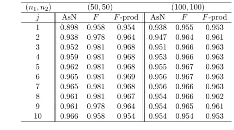
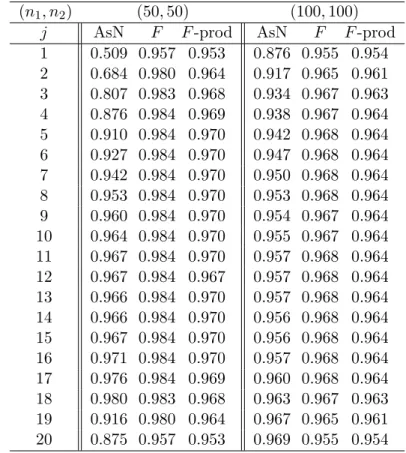
In Tables 2 and 3, we present the results for higher-dimensional cases for
p = 10, 20 than those of Table 1. We see that for larger and smaller
eigenval-ues, G(2)j is more accurate, whereas G(0)j is more accurate for eigenvalues of moderate size.
In the remaining tables, we present the results of simulations when n1̸= n2 for p = 5, 10, and 20. In Table 4, when (n1, n2) = (20, 50), we find that G(2)j
for j = 1, 2, 3, and 5 is the most precise of the three approximations. When (n1, n2) = (50, 20), G(2)j for j = 1, 2, 3 is the best of the three, and in the other cases, all three approximations have almost the same precision. In Table 5, when (n1, n2) = (10, 50) and (n1, n2) = (50, 20), we see that G(2)j is more
precise for the larger or smaller eigenvalues. The tendencies seen in Table 6 are similar to those seen in Table 5.
§4. Concluding remarks
In this paper, we consider the approximate distribution of the eigenvalues of a ratio of Wishart matrices, where each population has a single eigenvalue. Sugiura (1976) and Butler and Wood (2005) discussed the case of multiple eigenvalues, but we leave this for future work.
The authors would like to thank the editor and the anonymous reviewer for improving this paper. This research was supported in part by the Japan Society for the Promotion Science, Grant-in-Aid for Scientific Research (C), Nos. 25330033 and 26330053.
Table 1: Approximate distribution of the jth eigenvalue when p = 3
(n1, n2) (50, 50) (100, 100)
j Σ1Σ−12 AsN F F -prod AsN F F -prod
1 diag(6, 5, 1) 0.836 0.943 0.941 0.902 0.949 0.943 1 diag(6, 4, 1) 0.934 0.958 0.949 0.949 0.958 0.952 1 diag(6, 3, 1) 0.944 0.959 0.954 0.949 0.955 0.953 1 diag(6, 2, 1) 0.944 0.955 0.954 0.948 0.952 0.952 2 diag(6, 5, 4) 0.660 0.993 0.953 0.838 0.991 0.952 2 diag(7, 5, 4) 0.866 0.991 0.954 0.932 0.987 0.956 2 diag(8, 5, 4) 0.887 0.986 0.955 0.937 0.980 0.957 2 diag(6, 5, 3) 0.775 0.984 0.952 0.882 0.976 0.955 2 diag(6, 5, 2) 0.785 0.965 0.952 0.881 0.961 0.950 2 diag(6, 5, 1) 0.788 0.952 0.946 0.883 0.954 0.946 3 diag(6, 2, 1) 0.955 0.959 0.954 0.952 0.955 0.954 3 diag(6, 3, 1) 0.954 0.955 0.954 0.951 0.952 0.952 3 diag(6, 4, 1) 0.953 0.953 0.953 0.951 0.951 0.951 3 diag(6, 5, 1) 0.953 0.952 0.952 0.951 0.951 0.951
Table 2: Approximate distribution of the jth eigenvalue when p = 10 and Σ1Σ−12 = diag(29, 28, . . . , 20)
(n1, n2) (50, 50) (100, 100)
j AsN F F -prod AsN F F -prod
1 0.898 0.958 0.954 0.938 0.955 0.953 2 0.938 0.978 0.964 0.947 0.964 0.961 3 0.952 0.981 0.968 0.951 0.966 0.963 4 0.959 0.981 0.968 0.953 0.966 0.963 5 0.962 0.981 0.968 0.955 0.967 0.963 6 0.965 0.981 0.969 0.956 0.967 0.963 7 0.965 0.981 0.968 0.956 0.966 0.963 8 0.961 0.981 0.967 0.954 0.966 0.962 9 0.961 0.978 0.964 0.954 0.965 0.961 10 0.966 0.958 0.954 0.954 0.954 0.953 Note. AsN: G(0)j (x) F : G(1)j (x) F -prod: G(2)j (x)
Table 3: Approximate distribution of the jth eigenvalue when p = 20 and Σ1Σ−12 = diag(219, 218, . . . , 20)
(n1, n2) (50, 50) (100, 100)
j AsN F F -prod AsN F F -prod
1 0.509 0.957 0.953 0.876 0.955 0.954 2 0.684 0.980 0.964 0.917 0.965 0.961 3 0.807 0.983 0.968 0.934 0.967 0.963 4 0.876 0.984 0.969 0.938 0.967 0.964 5 0.910 0.984 0.970 0.942 0.968 0.964 6 0.927 0.984 0.970 0.947 0.968 0.964 7 0.942 0.984 0.970 0.950 0.968 0.964 8 0.953 0.984 0.970 0.953 0.968 0.964 9 0.960 0.984 0.970 0.954 0.967 0.964 10 0.964 0.984 0.970 0.955 0.967 0.964 11 0.967 0.984 0.970 0.957 0.968 0.964 12 0.967 0.984 0.967 0.957 0.968 0.964 13 0.966 0.984 0.970 0.957 0.968 0.964 14 0.966 0.984 0.970 0.956 0.968 0.964 15 0.967 0.984 0.970 0.956 0.968 0.964 16 0.971 0.984 0.970 0.957 0.968 0.964 17 0.976 0.984 0.969 0.960 0.968 0.964 18 0.980 0.983 0.968 0.963 0.967 0.963 19 0.916 0.980 0.964 0.967 0.965 0.961 20 0.875 0.957 0.953 0.969 0.955 0.954
Table 4: Approximate distribution of the jth eigenvalue when p = 5 and Σ1Σ−12 = diag(24, 23, . . . , 20)
(n1, n2) (20, 50) (50, 20)
j AsN F F -prod AsN F F -prod
1 0.937 0.960 0.954 0.836 0.956 0.951 2 0.964 0.985 0.963 0.935 0.986 0.962 3 0.965 0.985 0.963 0.956 0.988 0.967 4 0.958 0.986 0.962 0.962 0.985 0.963 5 0.969 0.956 0.951 0.953 0.960 0.954 Note. AsN: G(0)j (x) F : G(1)j (x) F -prod: G(2)j (x)
Table 5: Approximate distribution of the jth eigenvalue when p = 10 and Σ1Σ−12 = diag(29, 28, . . . , 20)
(n1, n2) (10, 50) (20, 50)
j AsN F F -prod AsN F F -prod
1 0.908 0.955 0.952 0.903 0.959 0.954 2 0.961 0.990 0.960 0.954 0.985 0.963 3 0.968 0.996 0.967 0.966 0.989 0.968 4 0.954 0.995 0.969 0.971 0.991 0.971 5 0.972 0.996 0.971 0.965 0.992 0.971 6 0.984 0.998 0.969 0.965 0.992 0.972 7 0.981 0.998 0.973 0.973 0.993 0.971 8 0.983 0.998 0.975 0.980 0.992 0.968 9 0.991 0.997 0.975 0.956 0.990 0.960 10 0.998 0.958 0.940 0.919 0.953 0.948
Table 6: Approximate distribution of the jth eigenvalue (j = 1, . . . , 20) when
p = 20 and Σ1Σ−12 = diag(219, 218, . . . , 20)
(n1, n2) (20, 50) (30, 50)
j AsN F F -prod AsN F F -prod
1 0.660 0.960 0.954 0.581 0.958 0.953 2 0.856 0.988 0.962 0.803 0.984 0.963 3 0.910 0.990 0.965 0.883 0.988 0.969 4 0.947 0.993 0.972 0.918 0.988 0.970 5 0.961 0.993 0.971 0.942 0.989 0.971 6 0.970 0.993 0.972 0.956 0.989 0.971 7 0.976 0.994 0.975 0.964 0.990 0.972 8 0.972 0.994 0.974 0.969 0.990 0.972 9 0.972 0.995 0.973 0.971 0.990 0.972 10 0.979 0.995 0.977 0.971 0.990 0.972 11 0.985 0.997 0.976 0.970 0.991 0.972 12 0.988 0.997 0.974 0.972 0.991 0.974 13 0.970 0.996 0.971 0.977 0.991 0.972 14 0.972 0.997 0.971 0.982 0.992 0.972 15 0.982 0.997 0.972 0.969 0.992 0.972 16 0.990 0.997 0.974 0.947 0.992 0.972 17 0.996 0.998 0.972 0.944 0.993 0.971 18 0.999 0.998 0.974 0.948 0.992 0.969 19 0.999 0.997 0.972 0.954 0.990 0.961 20 1.000 0.954 0.935 0.949 0.953 0.948 Note. AsN: G(0)j (x) F : G(1)j (x) F -prod: G(2)j (x)
References
[1] Butler, R. W. and Wood, A. T. A. (2005), Laplace Approximations to Hyperge-ometric Functions of Two Matrix Arguments, Journal of Multivariate Analysis,
94, 1–18.
[2] Chikuse, Y. (1977), Asymptotic Expansion for the Joint and Marginal Distribu-tions of the latent roots of S1S2−1, Annals of the Institute of Statistical
Mathe-matics, 29, 221–233.
[3] James, A. T. (1964), Distributions of Matrix Variates and Latent Roots Derived from Normal Samples, The Annals of Mathematical Statistics, 35, 475–501.
[4] Johnstone, I. M. (2001), On the Distribution of the Largest Eigenvalue in Prin-cipal Components Analysis, The Annals of Statistics, 29, 295–327.
[5] Johnstone, I. M. (2008), Multivariate Analysis and Jacobi Ensembles: Largest Eigenvalue, Tracy–Widom Limits and Rates of Convergence. The Annals of
Statistics, 36, 2638–2716.
[6] Johnstone, I. M. (2009), Approximate Null Distribution of the Largest Root in Multivariate Analysis, The Annals of Applied Statistics, 3, 1616–1633.
[7] Kato, H. and Hashiguchi, H. (2014), Chi-Square Approximation for Eigenvalue Distributions and Confidential Interval Construction on Population Eigenval-ues, Journal of the Japanese Society of Computational Statistics, 27, 11–28 (in Japanese).
[8] Khatri, C. G. (1967), Some Distribution Problems Connected with the Charac-teristic Roots of S1S2−1, The Annals of Mathematical Statistics, 38, 944–948.
[9] Khatri, C. G. (1972), On the Exact Finite Series Distribution of the Smallest or the Largest Root of Matrices in Three Situations, Journal of Multivariate
Analysis, 2, 201–207.
[10] Li, H. C., Pillai, K. C. S. and Chang, T. C. (1970), Asymptotic Expansions for Distributions of the Roots of Two Matrices from Classical and Complex Gaussian Populations, The Annals of Mathematical Statistics, 41, 1541–1556.
[11] Muirhead, R. J. and Chikuse, Y. (1975), Asymptotic Expansions for the Joint and Marginal Distributions of the Latent Roots of the Covariance Matrix, The
Annals of Statistics, 3, 1011–1017.
[12] Muirhead, R. J. (1982), Aspects of Multivariate Statistical Theory, John Wiley
& Sons, New York.
[13] Sugiura, N. (1973), Derivatives of the Characteristic Root of a Symmetric or a Hermitian Matrix with Two Applications in Multivariate Analysis,
[14] Sugiura, N. (1976), Asymptotic Expansion of the Distributions of the Latent Roots and the Latent Vector of the Wishart and Multivariate F Matrices, Journal
of Multivariate Analysis, 6, 500–525.
[15] Sugiyama, T. (1972), Approximation for the Distribution of the Largest Latent Root of a Wishart Matrix, The Australian Journal of Statistics, 14, 17–24. [16] Takemura, A. and Sheena, Y. (2005), Distribution of Eigenvalues and
Eigenvec-tors of Wishart Matrix when the Population Eigenvalues are Infinitely Dispersed and its Application to Minimax Estimation of Covariance Matrix, Journal of
Multivariate Analysis, 94, 271–299.
[17] Venables, W. (1973), Computation of the Null Distribution of the Largest or Smallest Latent Roots of a Beta Matrix, Journal of Multivariate Analysis, 3, 125–131.
Shusuke Matsubara
Graduate School of Mathematical Information Science, Tokyo University of Science 1-3 Kagurazaka, Shinjuku-ku, Tokyo, 162-8601, Japan
E-mail : [email protected]
Hiroki Hashiguchi
Department of Mathematical Information Science, Tokyo University of Science 1-3 Kagurazaka, Shinjuku-ku, Tokyo, 162-8601, Japan