Reactive n‑species Cahn Hilliard system: A thermodynamically‑consistent model for
reversible chemical reactions
Author S.P. Clavijo, A.F. Sarmiento, L.F.R. Espath, L. Dalcin, A.M.A. Cortes, V.M. Calo
journal or
publication title
Journal of Computational and Applied Mathematics
volume 350
page range 143‑154
year 2018‑10‑21
Publisher Elsevier
Rights (C)2018 Elsevier B.V.
Author's flag author
URL http://id.nii.ac.jp/1394/00001309/
doi: info:doi/10.1016/j.cam.2018.10.007
Creative Commons Attribution‑NonCommercial‑NoDerivatives 4.0
Reactive n-species Cahn–Hilliard System: A thermodynamically-consistent model for reversible chemical reactions
0SP Clavijo1,, AF Sarmiento2,, LFR Espath3,∗, L Dalcin4,, AMA Cortes5,, VM Calo1,6,7,
Curtin University, Bentley, Perth, Western Australia, Australia,
Okinawa Institute of Science and Technology Graduate University (OIST), Okinawa, Japan King Abdullah University of Science and Technology (KAUST), Thuwal, Saudi Arabia
Federal University of Rio de Janeiro, Rio de Janeiro, Brazil
Abstract
We introduce a multicomponent Cahn–Hilliard system with multiple reversible chemical reactions. We derive the conservation laws of the multicomponent system within the thermodynamical constraints. Furthermore, we consider multiple chemical reactions based on the mass action law. This coupling reproduces phase separation under spinodal decomposition as a chemical reaction between the species takes place. Finally, we perform a numerical simulation to show the robustness of the model as well as the resulting patterns.
Keywords: Multicomponent Cahn–Hilliard, Chemical Reactions, Isogeometric Analysis, Spinodal Decomposition
1. Introduction
Cahn and Hilliard [1] originally proposed a model that describes the phenomena associated with spon- taneous phase separation of immiscible fluids. Such processes occur below a critical temperature, where the phase separation forms spatial domains rich in each component. To date, modified versions of the model are widely used to describe biological entities [2, 3, 4], water filtration in porous media [5], wetting [6], image processing [7], binary alloys [8], and tumor-growth [9, 10, 11, 12]. An important open research topic in science and engineering is the evolution of multicomponent systems under spinodal decomposition.
Nonetheless, such an effort requires a comprehensive treatment that characterizes the dynamic behavior of each component as the system evolves. A generalized Cahn–Hilliard system, accounting for multiple phases, was first formulated by Morral and Cahn [13], and De Fontaine [14]. The generalized Cahn–Hilliard system is useful in materials science, particularly in alloy manufacturing, where the primary alloys used in engineer- ing structures have multiple phases in their microstructure. Additionally, in some specific applications, the
0© 2019. This manuscript version is made available under the CC-BY-NC-ND 4.0 license http://creativecommons.org/licenses/by-nc-nd/4.0/
∗Corresponding author.
Email address: [email protected](LFR Espath)
1Applied Geology, Western Australian School of Mines, Faculty of Science and Engineering, Curtin University, Perth, WA, Australia 6845
2Mathematics, Mechanics, and Materials Unit, Okinawa Institute of Science and Technology Graduate University, Onna, Okinawa 904-0495, Japan
3Computer, Electrical and Mathematical Sciences and Engineering, King Abdullah University of Science and Technology, Thuwal 23955-6900, Saudi Arabia
4Extreme Computing Research Center, King Abdullah University of Science and Technology, Thuwal 23955-6900, Saudi Arabia
5Federal University of Rio de Janeiro, RJ, 21941-901, Brazil
6Mineral Resources, Commonwealth Scientific and Industrial Research Organisation (CSIRO), Kensington, WA, Australia 61527Curtin Institute for Computation, Curtin University, Perth, WA, Australia 6845
microstructure may be the result of the phase transformation itself [15]. Thus, the generalized Cahn-Hilliard equation can model the kinetics of multicomponent systems and, most importantly, track the microstruc- ture evolution of the resulting phases to enhance the understanding of the resulting material properties. For instance, Honjo et al. [8], using the generalized Cahn-Hilliard equation, carried out a numerical simulation of phase separation in binary alloys as well as reviewed its extension towards ternary alloys. Hawkins et al. [16, 17], Gomez et al. [18], and Wu et al. [9] discussed this approach at length from a numerical point of view. Alternatively, the coupling of the Cahn-Hilliard equation with the law of mass action, allows one to model the spinodal decomposition and chemical reaction between the species. Modeling of the reactive Cahn-Hilliard equation has repeatedly been reported in the literature. For instance, Glotzer et al. [19] study a reversible chemical reaction that takes place simultaneously with spinodal decomposition. This interaction leads to a spatially periodic pattern when the demixing, caused by the diffusion, and the reactive mixing processes balance. Following this line, Christensen et al. [20] investigate steady-state pattern formation for a chemically reactive mixture that undergoes spinodal decomposition. The authors highlight the influence of the reaction rates upon the emerging pattern. Polymerization-induced phase segregation and its mor- phology can be described using the reactive Cahn-Hilliard equation whereby the chemical reaction inhibits the system evolution upon phase separation and restrict the domains rich in each component to microscopic length scale as suggested by Luo et al. [21]. Herein, we extend in a thermodynamically-consistent manner the Cahn-Hilliard reactive equation to include multicomponent systems. Elliot and Luckhaus [22] show the former Cahn-Hilliard equation can be recovered by assuming the gradient energy parameters matrix to be diagonal positive definite. We recover the Cahn-Hilliard equation using negative-definite gradient energy parameters with null diagonal. The outline of this work reads as follows. Section 2 defines of the free energy of the system. We use a logarithmic multi-well potential together with a multi-gradient-type potential. Sec- tion 3 introduces the expressions for the chemical potentials wherebyn−1 chemical potential differences are identified. Section 4 outlines the general expression for the mass flux taking into account the off-diagonal terms in the Onsager reciprocal relations, followed by sections 5 and 6, which encompass the governing equations and reaction terms of the diffusion-reaction process. In section 7, we carry out a theoretical anal- ysis of the first and second law of thermodynamics for the coupled multicomponent Cahn-Hilliard system with chemical reaction. The latter suggests the free energy may increase since the reaction term acts as a source/sink of energy. Finally, in section 8, we perform a simulation that showcases the evolution of a four phases system that undergoes a reversible chemical reaction. Particularly, when the forward reaction rate is greater than the backward one, we show the changes in interfacial energy.
2. Free Energy
We consider n-species, whereϕa denotes the concentration of the a-th species. The concentration of each species is linearly dependent on the others since
n
X
a=1
ϕa def= 1. (1)
To simplifly the notation, we define the following set of functions,
˜
ϕ={ϕ1, . . . , ϕn} (2a)
grad ˜ϕ={gradϕ1, . . . ,gradϕn} (2b)
ϕ={ϕ1, . . . , ϕn−1,1−
n−1
X
a=1
ϕa} (2c)
gradϕ={gradϕ1, . . . ,gradϕn−1,−
n−1
X
a=1
gradϕa} (2d)
where ˜ϕand grad ˜ϕaccount for the concentration of each component, and their gradients, respectively. The sets ϕ and gradϕ incorporate the constraint (1) by settingϕn = 1 - Pn−1
a=1ϕa , which is only possible in
the case of perfect mixture solutions. As a consequence, we rewrite the system without considering one of the species, for instanceϕn. The tilde stands for quantities evaluated on ˜ϕ and grad ˜ϕ.
As suggested by the pioneering work of Cahn and Hilliard[1], the nature of phase separation undergoing spinodal decomposition is governed by the Ginzburg-Landau free energy. In a multicomponent framework, we assume that the Ginzburg-Landau free energy for an isotropic physical domain Ω with a non-uniform concentration is
˜Ψ( ˜ϕ,grad ˜ϕ)def=Z
Ω
ψ( ˜˜ ϕ,grad ˜ϕ)dΩ =Z
Ω
ψ˜ϕ( ˜ϕ) + ˜ψs(grad ˜ϕ)dΩ, (3) where ˜ψϕ and ˜ψs are the specificn-well and interfacial free energies. Then-well free energy is
ψ˜ϕ( ˜ϕ) =NvkBθ
n
X
a=1
ϕalnϕa
! +Nv
n
X
a=1 n
X
b=1
ωabϕaϕb (4a)
ψϕ(ϕ) =NvkBθ
n−1
X
a=1
ϕalnϕa+ (1−
n−1
X
a=1
ϕa) ln(1−
n−1
X
b=1
ϕb)
!
+Nv n−1
X
a=1 n−1
X
b=1
(ωab+ωnn−ωan−ωnb)ϕaϕb+n−1X
a=1
(ωan+ωna−2ωnn)ϕa
!
(4b) where Nv is the number of molecules per unit volume, kB is the Boltzmann constant, andωab represents the interaction energy between the mass fraction of the species a and b, where the interaction between the phaseϕa overϕbis reciprocal, thusωabis symmetric. The interaction energy is positive and is related to the critical temperature for each pair of species,θcab, (between phasesaandb). Following standard convention, we assumeωab= 0 when a=b andωab=kBθcabwhena,b[23, 22, 24, 25, 26].
The interfacial free energy is defined as ψ˜s(grad ˜ϕ) =1
2
n
X
a=1 n
X
b=1
γabgrad (ϕa)·grad (ϕb) (5a)
ψs(gradϕ) =1 2
n−1
X
a=1 n−1
X
b=1
(γab+γnn−γan−γnb)grad (ϕa)·grad (ϕb) (5b) where γab=σablab[force] (no summation implied by repeated indexes) represents the magnitude of the interfacial energy between the phases ϕa and ϕb. The parameters σab and lab are the interface tension [force/length] and the interfacial thickness8 for each pair of species (between phases ϕa and ϕb) [length], respectively. In [27], the authors define the forceγabasNvωablab2 . For example, from the previous expressions we can recover the Cahn-Hilliard equation by settingn= 2 andγab=−0.5γfora,bandγab= 0 fora=b.
We then show the Cahn-Hilliard equation can also be recovered using a negative definite gradient energy parameters with null diagonal. Similarly forω, keeping the same structure as γ, ωab =ω/2 fora,b and ωab= 0 fora=b.
Applying the constraint (1) to the equations (4a) and (5a), we obtain a new form for the free energies, which is given in the equations (4b) and (5b), respectively.
Remark 1 (The nature ofγab).Letλab be a fully populated matrix with the same entity, κfor all aand b. Given the constraint
n
X
a=1
ϕa= 1⇒
n
X
a=1
gradϕa = 0a, (6)
8This expression corresponds to the root mean square effective ”interaction distance,” as suggested by the former work of Cahn and Hilliard [27].
the inner product between the rows (which are constant for this particular case) and the gradϕ is always zero. Thus, gradϕis the null space (kernel) ofλab, i.e., Null(λab) =gradϕ. We thus arrive at
n
X
a=1 n
X
b=1
gradϕaγabgradϕb=
n
X
a=1 n
X
b=1
gradϕa(γab+λab)gradϕb. (7) We conclude then that any statement about the positive definiteness ofγab could be misleading.
Conversely, if we impose the constraint on the last componentn, in the following quadratic form
n
X
a=1 n
X
b=1
gradϕaγabgradϕb, (8)
we arrive at
n
X
a=1 n
X
b=1
gradϕaγabgradϕb=n−1X
a=1 n−1
X
b=1
gradϕa(γab+γnn−γan−γnb
| {z }
¯ γab
)gradϕb. (9)
That is, this results in an unconstrained space of dimensionn−1 with the mappingF:γ7→¯γdefined by
¯
γab=γab+γnn−γan−γnb, for1≤a, b≤n−1. (10) We thus postulate that the problem is well-posed if¯γab is positive-definite. Moreover, γabcan be positive- or negative-definite.
Moreover, letea be a basis (of a vector spaceV) of dimension n,eˆa be a basis (in the dual spaceV∗), andγabbe a diagonal matrix defined as follows
γab=κˆea·eb. (11)
γabcan be rewritten as
γab=−κ(1−eˆa·eb). (12)
Although the matrix (12)has a null diagonal, it produces the same mapping as the diagonal matrix (11) for all vectors that live in the constrained vector space.
3. Chemical potential
The conserved field obeys a non-Fickian diffusion driven by the chemical potential differences between the species. The chemical potential is the variational derivative of the free energy functional with respect to the selected species concentration, and models the n-well and interfacial contributions to the exchange process. We assume that the chemical potential in a multicomponent system is
˜ ηa
def= δ˜Ψ δϕa
. (13)
Then, we obtain that
δΨ δϕa
def= δ˜Ψ δϕa − δ˜Ψ
δϕn
= ˜ηa−η˜n, (14)
fora= 1, . . . , n−1.
As mentioned above, we split the chemical potential into the n-well ηϕ and interfacial ηs chemical potentials, related to then-well and interfacial free energies, respectively. Then-well term is
˜
ηϕa =Nvkθ(lnϕa+ 1) +Nv n
X
b=1
(ωab+ωba)ϕb
=Nvkθ(lnϕa+ 1) + 2Nv n
X
b=1
ωabϕb, (15a)
whereas the interfacial one is
˜ ηas=−1
2
n
X
b=1
(γab+γba)4ϕb
=−
n
X
b=1
γab4ϕb. (16a)
Applying the relation (14), the chemical pontentials read ηaϕ=Nvkθ
ln ϕa
ϕn
+ 2Nv n
X
b=1
(ωab−ωnb)ϕb, (17)
and
ηas=−
n
X
b=1
(γab−γnb)4ϕb. (18)
Finally,ηa def= ηϕa +ηsa.
4. Generalized Fick’s law
We consider the off-diagonal terms in the Onsager reciprocal relations and thus, we describe the mass fluxes as
jadef= −
n
X
b=1
Labgrad ˜ηb, a= 1, . . . , n, (19) whereLabare the Onsager mobility coefficients. To conserve mass, we must guarantee that the mass fluxes satisfy
n
X
a=1
ja= 0, (20)
which implies the relation
n
X
b=1
Lab= 0, ∀a. (21)
Finally, the mass flux for each component is ja =−
n
X
b=1
Labgrad ˜ηb
=−
n−1
X
b=1
Labgrad ˜ηb+Langrad ˜ηn
!
=−
n−1
X
b=1
Labgrad ˜ηb−(n−1X
b=1
Lab) grad ˜ηn
!
=−
n−1
X
b=1
Labgrad (˜ηb−η˜n)
(22)
We use the standard assusmption that the mobility coefficients depend on the phase composition. In particular, we express this dependency in terms of the concentration of each species. We use the definition Lab=ϕa(δab−ϕb) with no sum onaand b, whereδabis the Kronecker delta of dimension n[23]. Finally, the mass flux is
ja=−
n−1
X
b=1
Labgradηb, (23)
5. Mass action law
We express a general chemical reaction as
n
X
a=1
αaAa k+ k−
n
X
a=1
βaAa, (24)
where the number of reactants and the number of products are given by the number of non-zero entries in αa andβa [28]. The stoichiometry coefficients αa and βa balance the chemical reaction andk− andk+ account for the reaction rates in the forward and backward reactions, respectively. Aa stands for the species in the forward and backward chemical equations. As mentioned above,n corresponds to the total number of species involved in the chemical process. For instance, if one considers the formation of water from its elements, hydrogen and oxygen, the chemical reaction reads
2H2(g) +O2(g)→2H2O(g). (25)
Using equation (24) to describe the aforementioned chemical reaction, the total number of species corre- sponds ton = 3 and the chemical speciesA1, A2 and A3 relates H2(g), O2(g) andH2O(g), respectively.
Moreover, the stoichiometry coefficients in left-hand side of the chemical reaction are given by (α1, α2, α3)
= (2, 1, 0). Analogously, the stoichiometry coefficients in the right-hand side of the chemical reaction are (β1, β2, β3) = (0,0,2).
Consider now the mass fractions of thea-th speciesAadenoted by [Aa], with ˜ϕdef= [Aa], i.e., (ϕ1, . . . , ϕn)def= ([A1], . . . ,[An]). Hence, the forward reaction rate, defined by the law of mass action, states that
r+ def= k+
n
Y
a=1
[Aa]αa=k+
n
Y
a=1
ϕαaa, (26)
while, the backward reaction rate
r−def= k−
n
Y
a=1
[Aa]βa=k−
n
Y
a=1
ϕβaa. (27)
For convenience, we rewrite the general reaction term as follows:
Ra=−(αa−βa)(r+c −r−c ), (28) and to consider multiplensgeneral reactions, we define
rc+def= kc+
n
Y
a=1
ϕαaac, (29)
r−c def= k−c
n
Y
a=1
ϕβaac, (30)
Ra=−
ns
X
c
(αac−βac)(rc+−rc−), (31)
where αac and βac are the a-th are the stoichiometry coefficient (with the index a for each component) for the c-th chemical reaction, while k+c and k−c are the forward and backward reaction rates for the c-th chemical reaction, respectively.
6. Governing Equations in Primal Form
The temporal evolution of the conserved field undergoing spinodal decomposition with chemical reaction is governed by
˙
ϕa =Ra−divja for each species a. (32)
We denoteH2as the Sobolev space of square integrable functions with square integrable first and second derivatives and (·,·)Ωas theL2inner product over the physical domain Ω with boundary Γ. By multiplying the governing equation (32) by a test functionwa, which belongs toH2, using the definition for the mass fluxes (19) and integrating by parts, the primal variational formulation can then be given by:
(%a,ϕ˙a)Ω=(%a,Ra)Ω−(%a, ∂ijai)Ω
=(%a,Ra)Ω+ (∂i%a, jai)Ω−(%a, jaini)Γ
=(%a,Ra)Ω+ (∂i%a,−Lab∂i(ηbϕ+ηbs))Ω−(%a,−Lab(∂iηb)ni)Γ
=(%a,Ra)Ω−(∂i%a, Lab∂iηϕb)Ω−(∂i%a, ∂i(Labηbs))Ω+ (∂i%a,(∂iLab)ηbs)Ω
+ (%a, Lab(∂iηb)ni)Γ
=(%a,Ra)Ω−(∂i%a, Lab∂iηϕb)Ω+ (∂ii%a, Labηsb)Ω+ (∂i%a,(∂iLab)ηbs)Ω
+ (%a, Lab(∂iηb)ni)Γ−(∂i%ani, Labηsb)Γ
(33)
7. First and second law of thermodynamics
We derive the first law of thermodynamics using the governing equation of mass evolution. The product between the temporal derivative of the concentration and the chemical potential yields the balance between the external and internal chemical powers provided by diffusion. Additionally, the product between the chemical potential and the law of mass action accounts for the chemical power provided by the chemical reaction. We assume the following dependence on the free energy and chemical powers
˙
wint=Xn
a
∂ϕaψ˜ϕ˙a+∂gradϕaψ˜·grad ˙ϕa−gradηa·ja
, (34a)
˙ wext=
n
X
a
(−div (ηaja−ϕ˙aγgradϕa)−ηaRa), (34b) where ˙wint and ˙wext stand for the internal and external chemical powers, respectively, cf. [29, 30]. Thus, the governing equation yields ˙wint= ˙wext.
When considering the free energy in the form (3), i.e., ˜ψdef= ˜ψ[ϕ,gradϕ] the total derivative of the energy functional reads
ψ˙˜=
n
X
a
∂ϕaψ˜ϕ˙a+∂gradϕaψ˜·grad ˙ϕa (35) which leads to ˙wint= ˙˜ψ−Pn
a(gradηa·ja).
The first law of thermodynamics accounts for the energy balance between the internal energy ˙eint and the rate at which chemical (diffusion and reaction) power is expended ˙wext. Thereby, the latter statement leads to the following expression
˙
eint= ˙˜ψ−
n
X
a
(gradηa·ja). (36)
The second law of thermodynamics, in the form of the Clausius-Duhem inequality, states that the rate of growth of the entropysis at least as large as the entropy fluxq/θ added to the entropy supplyq/θ, i.e.,
˙ s≥ 1
θ(−divq+1
θdivθ·q+q) (37)
where q, q and θ stand for heat flux, heat supply, and temperature, respectively. Using the Legrende transform of the free energy and taking the temporal derivative of the resulting expression, we end up with the following expression
ψ˙˜= ˙eint−θs˙ −θs,˙ (38)
and considering the absence of a heat flux, the entropy imbalance reads
˙
eint−ψ˙˜≥0 (39)
which follows from combining (38) and (37). Finally, the entropy inequality reads
−
n
X
a
(gradηa·ja)≥0 (40)
8. Numerical Simulations
We perform a numerical simulation of a two-dimensional multicomponent Cahn-Hilliard reactive equation that showcases the temporal evolution and interactions of a four species system A1, A2, A3 and A4 as expressed by the model we propose in the previous sections. Herein, we consider a reversible chemical reaction with forward k+ and backward k− reaction rates of 1000 and 10, respectively. The chemical reaction in our formulation is general. Therefore, modeling a specific chemical process does not generate neither implementation nor theoretical difficulties. By inserting the corresponding stoichiometry coefficients and reaction rates, our model is capable of representing arbitrary processes. We consider the following chemical reaction,
5A1+A2k+
k− 2A3+A4, (41)
where the stoichiometry vectorsαa andβa are given by
αa= (5,1,0,0), and βa= (0,0,2,1). (42)
In a reversible chemical reaction, the reactant and product species are never totally consumed. For instance, in equation (41), the speciesA1 andA2 react to form the species A3 andA4which in turn react to form back the species A1 and A2 until the system reaches equilibrium. In general, such reactions do not need to have the same reaction rates. Thereby, we seek to model a system which follows a reversible chemical reaction such as (41).
Regarding the physical parameters that rule the spinodal decomposition, we set the interaction energy as
ωab=
0.0 0.5 0.7 0.6 0.5 0.0 0.4 0.7 0.7 0.4 0.0 0.7 0.6 0.7 0.7 0.0
(43)
Moreover, the magnitude of the interfacial energy between ϕa andϕb is
γab=
0.0 −0.5 −0.75 −0.75
−0.5 0.0 −0.45 −0.65
−0.75 −0.45 0.0 −0.75
−0.75 −0.65 −0.75 0.0
(44)
For instance, the magnitude of the interfacial energy betweenϕ1 andϕ3 corresponds to−0.75.
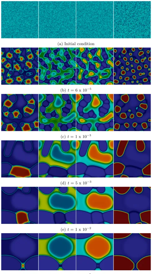
The parameters NvkBθand Nv take the values of 9000 and 6000, respectively. Furthermore, the initial condition for each component is set such that ϕa takes random values between ¯ϕa ±0.05, assuming that
¯
ϕa is 1/n. As discussed above, we calculateϕn by applying at each time-step the constraint defined by (1), which guarantees the consistency of the process. The coupled system of partial differential equations for our
(a) Initial condition
(b)t= 6 x 10⁻⁵
(c)t = 1 x 10⁻³
(d)t= 5 x 10⁻³
(e)t = 1 x 10⁻²
(f)t= 3 x 10⁻²
Figure 1: Temporal evolution of the concentration for species 1, 2, 3 and, 4, respectively.
example computes four coupled concentrations corresponding to [Aa] =ϕa, for a= 1, . . . ,4, that evolve in time, is
˙
ϕ1=−5k+ϕ51ϕ2+ 5k−ϕ23ϕ4−divj1, (45a)
˙
ϕ2=−k+ϕ51ϕ2+k−ϕ23ϕ4−divj2, (45b)
˙
ϕ3= 2k+ϕ51ϕ2−2k−ϕ23ϕ4−divj3, (45c)
˙
ϕ4=k+ϕ51ϕ2−k−ϕ23ϕ4−divj4, (45d) We form and solve the system of equations using PetIGA [31], an open soure framework for high- performance computing which has proven flexible, robust and highly scalable. This framework was applied to various multiphysics and multiscale proceeses, in particular phase-field modeling applications [32, 33, 34, 35, 29, 36, 17, 37, 30]. Following [18], we use isogeometric analysis to discretize in space equation (33). This technique successfully solves the standard Cahn–Hilliard equation in primal form as it allows for high-order, and highly-continuous basis functions, i.e., H2-conforming spaces. We use a square domain Ω = [0,1]2, using 64C1-quadratic elements with periodic boundary conditions. In order to control possible numerical instabilities induced by the time discretization, we use the generalized-αmethod as suggested by Vignal et al. [38].
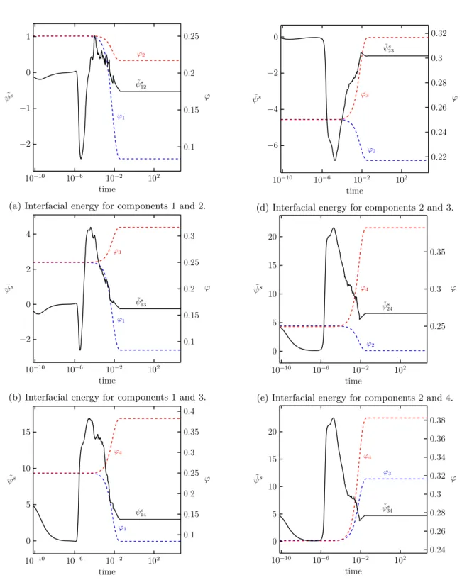
Figure 1 presents the temporal evolution of the concentration of each component. The randomly per- turbed initial condition goes through spinodal decomposition during the early stages and is followed by coarsening. Our results highlight these phenomena including the reaction process. Figures 1b and 1c depict the early stages of the process,t <10−3, when chain structures are formed by components 1 and 4, whereas the components 2 and 3 play an interstitial role. Later on,t >10−3, a merging process takes place to form large and rounded structures. When the system reaches steady state, the component 1 forms a bridge at the interface of the two elliptical structures defined by component 4. Furthermore, the component 2 becomes the interstitial component, while the component 3 forms a circular structure, surrounded by the component 4. Figure 2 depicts the interfacial energy pair (solid black lines) and the masses of each component (red and blue dashed lines). The chemical reactions occur mainly in the range 10−3 < t < 10−2, and outside this range the mass of each component remains roughly constant. Since the backward reaction plays no substantial role in the process, due to the fact thatk+ >> k−, components 1 and 2 react decreasing their initial masses. Consequently, this reaction increases the masses of the components 3 and 4 as a function of the consumption of reactant components. The nature of a system undergoing chemical reactions can create (destroy) the interface between the phases. Thus, the interfacial energy must also change according to this evolution process. Particularly, Figure 2d illustrates this process, whereby the interfacial energy grows as a result of the emerging product phase. On the contrary, when considering the early stages of each phase, Figure 2 suggests that the spinodal decomposition controls the interfacial energy evolution since the chemical process plays no substantial role during this early process. The relation between the free-energy and the external power, ˙˜ψ−Pn
a(gradηa ·ja) = ˙wext, bearing in mind that the use periodic boundary conditions renders ˙wext=−Pn
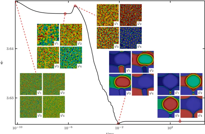
aηaRa, suggests the reaction term may act as either source or sink of energy, explaining the growth observed in the free-energy. Therefore, this reaction may increase the free energy. Figure 3 provides a picture of such behavior.
The spinodal decomposition controls the early stages since the phases start separating (unmixing) from each other. Later on, the system favors the growth of regions rich in each component caused by either phase merging or Ostwald ripening. Figure 3 shows the evolution over time of the total free-energy functional depicting the concentration fields at four stages, that is, the initial condition, spinodal decomposition, coarsening at the beginning of the chemical reaction, at the end of the chemical reaction, and the steady state.
0.1 0.15 0.2 0.25 ϕ2
ψ˜12s
ϕ1
ϕ
10−10 10−6 10−2 102
−2
−1 0 1
time ψ˜s
(a) Interfacial energy for components 1 and 2.
0.1 0.15 0.2 0.25 0.3 ϕ3
ψ˜13s ϕ1
ϕ
10−10 10−6 10−2 102
−2 0 2 4
time ψ˜s
(b) Interfacial energy for components 1 and 3.
0.1 0.15 0.2 0.25 0.3 0.35 0.4
ϕ4
ψ˜14s ϕ1
ϕ
10−10 10−6 10−2 102 0
5 10 15
time ψ˜s
(c) Interfacial energy for components 1 and 4.
0.22 0.24 0.26 0.28 0.3 0.32
ϕ3 ψ˜s23
ϕ2
ϕ
10−10 10−6 10−2 102
−6
−4
−2 0
time ψ˜s
(d) Interfacial energy for components 2 and 3.
0.25 0.3 0.35
ϕ4 ψ˜24s
ϕ2
ϕ
10−10 10−6 10−2 102 0
5 10 15 20
time ψ˜s
(e) Interfacial energy for components 2 and 4.
0.24 0.26 0.28 0.3 0.32 0.34 0.36 0.38 ϕ4
ψ˜34s ϕ3
ϕ
10−10 10−6 10−2 102 0
5 10 15 20
time ψ˜s
(f) Interfacial energy for components 3 and 4.
Figure 2: Temporal evolution of interfacial energy and mass.
10−10 10−6 10−2 102 3.63
3.64
time Ψ˜
Figure 3: Temporal evolution of free energy.
9. Conclusions
We derive a set of conservation laws within the appropriate thermodynamic constraints for a multicom- ponent Cahn–Hilliard system with multiple reversible chemical reactions. For binary systems, we recover the standard Cahn–Hilliard equation. Additionally, we couple the multi-phase framework with chemical reactions using the mass action law. We perform a numerical simulation with four components and one re- versible chemical reaction with different chemical reaction rates that showcases the robustness of the model we propose. The simulation also shows consistency with expected spinodal decomposition as well as the reversible chemical reaction.
10. Acknowledgments
This publication was made possible in part by the CSIRO Professorial Chair in Computational Geoscience at Curtin University and the Deep Earth Imaging Enterprise Future Science Platforms of the Commonwealth Scientific Industrial Research Organisation, CSIRO, of Australia. Additional support was provided by the European Union’s Horizon 2020 Research and Innovation Program of the Marie Skłodowska-Curie grant agreement No. 777778, and the Mega-grant of the Russian Federation Government (N 14.Y26.31.0013).
Additional, support was provided at Curtin University by The Institute for Geoscience Research (TIGeR) and by the Curtin Institute for Computation. The J. Tinsley Oden Faculty Fellowship Research Program at the Institute for Computational Engineering and Sciences (ICES) of the University of Texas at Austin has partially supported the visits of VMC to ICES.
References
[1] J. W. Cahn, J. E. Hilliard, Free energy of a nonuniform system. I. Interfacial free energy, The Journal of Chemical Physics 28 (2) (1958) 258–267.
[2] E. Khain, L. M. Sander, Generalized Cahn-Hilliard equation for biological applications, Physical Review E 77 (5) (2008) 051129.
[3] E. L. Elson, E. Fried, J. E. Dolbow, G. M. Genin, Phase separation in biological membranes: integration of theory and experiment, Annual review of biophysics 39 (2010) 207–226.
[4] L. Cherfils, A. Miranville, S. Zelik, On a generalized Cahn-Hilliard equation with biological applications, Discrete &
Continuous Dynamical Systems-Series B 19 (7).
[5] H. Gomez, L. Cueto-Felgueroso, R. Juanes, Three-dimensional simulation of unstable gravity-driven infiltration of water into a porous medium, Journal of Computational Physics 238 (2013) 217–239.
[6] L. Cueto-Felgueroso, R. Juanes, Macroscopic phase-field model of partial wetting: bubbles in a capillary tube, Physical review letters 108 (14) (2012) 144502.
[7] A. L. Bertozzi, S. Esedoglu, A. Gillette, Inpainting of binary images using the Cahn-Hilliard equation, IEEE Transactions on image processing 16 (1) (2007) 285–291.
[8] M. Honjo, Y. Saito, Numerical simulation of phase separation in Fe-Cr binary and Fe-Cr-Mo ternary alloys with use of the Cahn-Hilliard equation, ISIJ international 40 (9) (2000) 914–919.
[9] X. Wu, G. Zwieten, K. Zee, Stabilized second-order convex splitting schemes for Cahn-Hilliard models with application to diffuse-interface tumor-growth models, International journal for numerical methods in biomedical engineering 30 (2) (2014) 180–203.
[10] S. M. Wise, J. S. Lowengrub, H. B. Frieboes, V. Cristini, Three-dimensional multispecies nonlinear tumor growth—i:
model and numerical method, Journal of theoretical biology 253 (3) (2008) 524–543.
[11] H. Garcke, K. F. Lam, E. Sitka, V. Styles, A cahn-hilliard-darcy model for tumour growth with chemotaxis and active transport, Mathematical Models and Methods in Applied Sciences 26 (06) (2016) 1095–1148.
[12] P. Colli, G. Gilardi, E. Rocca, J. Sprekels, Optimal distributed control of a diffuse interface model of tumor growth, Nonlinearity 30 (6) (2017) 2518.
[13] J. Morral, J. Cahn, Spinodal decomposition in ternary systems, Acta metallurgica 19 (10) (1971) 1037–1045.
[14] D. De Fontaine, A computer simulation of the evolution of coherent composition variations in solid solutions, University Microfilms, 1978.
[15] Y. Li, J.-I. Choi, J. Kim, Multi-component Cahn-Hilliard system with different boundary conditions in complex domains, Journal of Computational Physics 323 (2016) 1–16.
[16] A. Hawkins-Daarud, K. G. van der Zee, J. Tinsley Oden, Numerical simulation of a thermodynamically consistent four- species tumor growth model, International journal for numerical methods in biomedical engineering 28 (1) (2012) 3–24.
[17] P. Vignal, L. Dalcin, N. O. Collier, V. M. Calo, Modeling phase-transitions using a high-performance, isogeometric analysis framework, Procedia Computer Science 29 (2014) 980–990.
[18] H. G´omez, V. M. Calo, Y. Bazilevs, T. J. Hughes, Isogeometric analysis of the Cahn-Hilliard phase-field model, Computer methods in applied mechanics and engineering 197 (49) (2008) 4333–4352.
[19] S. C. Glotzer, A. Coniglio, Self-consistent solution of phase separation with competing interactions, Physical Review E 50 (5) (1994) 4241.
[20] J. J. Christensen, K. Elder, H. C. Fogedby, Phase segregation dynamics of a chemically reactive binary mixture, Physical Review E 54 (3) (1996) R2212.
[21] K. Luo, The morphology and dynamics of polymerization-induced phase separation, European polymer journal 42 (7) (2006) 1499–1505.
[22] C. M. Elliott, S. Luckhaus, A generalised diffusion equation for phase separation of a multi-component mixture with interfacial free energy, Tech. rep., Institute for Mathematics and its Applications, IMA preprint series # 887 (1991).
[23] C. M. Elliott, H. Garcke, Diffusional phase transitions in multicomponent systems with a concentration dependent mobility matrix, Physica D: Nonlinear Phenomena 109 (3) (1997) 242–256.
[24] M. E. Gurtin, On a nonequilibrium thermodynamics of capillarity and phase, Quarterly of applied mathematics 47 (1) (1989) 129–145.
[25] J. Hoyt, The continuum theory of nucleation in multicomponent systems, Acta Metallurgica et Materialia 38 (8) (1990) 1405–1412.
[26] F. Boyer, C. Lapuerta, Study of a three component cahn-hilliard flow model, ESAIM: Mathematical Modelling and Numerical Analysis 40 (4) (2006) 653–687.
[27] J. W. Cahn, J. E. Hilliard, Free energy of a nonuniform system. III. Nucleation in a two-component incompressible fluid, The Journal of chemical physics 31 (3) (1959) 688–699.
[28] K. Fellner, B. Q. Tang, Explicit exponential convergence to equilibrium for nonlinear reaction-diffusion systems with detailed balance condition, Nonlinear Analysis: Theory, Methods & Applications.
[29] L. Espath, A. Sarmiento, P. Vignal, B. Varga, A. Cortes, L. Dalcin, V. Calo, Energy exchange analysis in droplet dynamics via the Navier-Stokes-Cahn-Hilliard model, Journal of Fluid Mechanics 797 (2016) 389–430.
[30] L. Espath, A. Sarmiento, L. Dalcin, V. Calo, On the thermodynamics of the Swift-Hohenberg theory, Continuum Mechanics and Thermodynamics (2017) 1–11.
[31] L. Dalcin, N. Collier, P. Vignal, A. Cˆortes, V. M. Calo, Petiga: A framework for high-performance isogeometric analysis, Computer Methods in Applied Mechanics and Engineering 308 (2016) 151–181.
[32] P. Vignal, L. Dalcin, D. L. Brown, N. Collier, V. M. Calo, An energy-stable convex splitting for the phase-field crystal equation, Computers & Structures 158 (2015) 355–368.
[33] A. M. Cˆortes, A. L. Coutinho, L. Dalcin, V. M. Calo, Performance evaluation of block-diagonal preconditioners for the divergence-conforming b-spline discretization of the stokes system, Journal of Computational Science 11 (2015) 123–136.
[34] P. Vignal, A. Sarmiento, A. M. Cˆortes, L. Dalcin, V. M. Calo, Coupling navier-stokes and Cahn-Hilliard equations in a two-dimensional annular flow configuration, Procedia Computer Science 51 (2015) 934–943.
[35] A. F. Sarmiento, A. M. Cˆortes, D. Garcia, L. Dalcin, N. Collier, V. M. Calo, Petiga-mf: a multi-field high-performance toolbox for structure-preserving b-splines spaces, Journal of Computational Science 18 (2017) 117–131.
[36] A. M. Cˆortes, P. Vignal, A. Sarmiento, D. Garc´ıa, N. Collier, L. Dalcin, V. M. Calo, Solving nonlinear, high-order partial differential equations using a high-performance isogeometric analysis framework, in: Latin American High Performance Computing Conference, Springer, 2014, pp. 236–247.
[37] A. Sarmiento, D. Garcia, L. Dalcin, N. Collier, V. Calo, Micropolar fluids using b-spline divergence conforming spaces, Procedia Computer Science 29 (2014) 991–1001.
[38] P. Vignal, N. Collier, L. Dalcin, D. Brown, V. Calo, An energy-stable time-integrator for phase-field models, Computer Methods in Applied Mechanics and Engineering 316 (2017) 1179–1214.