Copyright@SPSD Press from 2010, SPSD Press, Kanazawa
Modelling Spatial Distribution of Outdoor Recreation Trips of Urban Residents
An in-depth study in Salford, UK
Xihe Jiao1*, Ying Jin1, Oliver Gunawan2 and Philip James2
1 Archituecture Department, University of Cambridge
2 School of Environment and Life Sciences, Peel Building, University of Salford
* Corresponding Author, Email: [email protected] Received 3 April, 2014; Accepted 24 November, 2014
Key words: Spatial distribution, outdoor recreation travel, travel demand modelling, urban greenspaces, GIS.
Abstract: Outdoor recreation is one of the most important leisure activities of urban residents, with urban greenspace accruing the highest value of benefits among all greenspaces in the UK. However, access and trip-making to outdoor greenspaces by urban residents remain poorly understood. Existing trip- making prediction models that have been established for assessing the recreation benefits of outdoor greenspaces have dealt separately with visits to urban and rural greenspaces. This makes it difficult to assess greenspace strategies when considering them as a whole infrastructure. Meanwhile there is a risk of misjudging the value (e.g. double counting) when they are summed mechanically. This research aims to investigate the strengths and weaknesses of predictive models of outdoor recreation travel. An output of the research is a new model with two components: (a) predominantly local trips and (b) predominantly non-local trips. The resultant model is able to make an assessment that seamlessly combines urban and rural greenspaces. It also links the spatial distribution of visits to key spatial factors, such as distribution of population, location of recreational sites, transport accessibility and travel time. The resulting quantification of the impacts of policy interventions provide a robust basis for decision making
1. INTRODUCTION
Greenspace generates a wide range of valuable ecosystem services in urban areas. Outdoor recreation is one of the most important leisure activities of the urban residents, with urban greenspace accruing the highest value of benefits among all greenspaces in the UK (Natural England, 2013). In a recent survey from Nature England (2013) it is estimated that 2,858 million outdoor recreational visits were made in England during 2012, entailing direct expenditure of over £20 billion. The main benefits include recreation, aesthetics, and improved physical and mental health (Davis et al., 2011), yet land-use decisions often ignore the value of these services (Bateman, 2013). However, access and trip-making to outdoor greenspaces by urban residents remain poorly understood. In particular, travel prediction models used for transport planning purposes tend not to focus on access and travel to outdoor spaces; there is a resultant lack of precision in trip-making predictions; on the other hand, trip- making prediction models (for example, the UK National Ecosystem Assessment/NEA) that have been established for assessing the recreation benefits of outdoor greenspaces distinguish between visits to urban greenspaces and those to outside cities or towns. The separation of destinations makes the
36
prove that either people’s choice of outdoor recreational destinations nor greenspace planning/design strategies’ intent indicate that urban and rural areas should be treated separately. It would be useful to have a method that is able to assess consistently the benefits regarding the spatial distribution of the greenspaces. Meanwhile, the existing valuation methods have very limited spatial granularity, particularly in urban areas; this limits their use in local studies.
In this research a logit discrete choice model was used, which has been widely recognised in the transport planning area, and new predictive model was developed with two components: (a) predominantly local trips, and (b) predominantly non-local trips. This method allowed the prediction of the number of trips continually in the sense of spatial distributions. Meanwhile, site location, size and some other social-demographic characteristics were linked with a prediction of the number of trips. The resultant model had significantly improved capabilities in assessing policy interventions regarding allocation and design of urban greenspaces.
The main research questions we aim to answer in this paper are:
1) Existing models in UK NEA (Sen, et al., 2013; Perino et al., 2011) deal separately with (a) visits to urban greenspaces and (b) those to rural areas, while people’s choices are continuous in space – can the two models be integrated into one to reflect destination choice behaviour?
2) Existing models have very limited spatial granularity which limits their use in local studies – can the model incorporate more local details through applying travel demand modelling techniques?
The remainder of this paper is organised as follows. Section 2 is reviewing the exiting research related to outdoor recreational value and the discrete choice modelling. Section 3 contains a description of the data and the empirical methodology for building the trip prediction model. In Section 4 the model results are set out and in section 5 the manuscript concludes with an evaluation of the future works for this research. We aim to develop a new predictive model, which can estimate the outdoor recreational behaviour consistently. It will improve significantly the capabilities of choice modelling in assessing policy interventions regarding allocation and design of urban greenspaces.
2. LITERATURE REVIEW
2.1 Existing outdoor recreational value models
The Millennium Ecosystem Assessment (2005) not only demonstrated the importance of ecosystem services to human well-being, but also showed that at the global scale many key services are being degraded and lost. As a result, in 2007 the House of Commons Environmental Audit recommended that the Government should conduct a full Millennium Ecosystem Assessment type assessment for the UK to enable the identification and development of effective policy responses to ecosystem service degradation. The resultant UK National Ecosystem Assessment (UK NEA) was the first analysis of the UK’s natural environment in terms of the benefits it provides to society and continuing economic prosperity.
Many previous studies for recreational sites focus on either single habitat recreational sites (Public Opinion of Forestry, 2013; Inland Waterways Visits Survey, 2013; National Park Visitor Survey, etc.) or on a particular type of activity (Great Britain Tourism Survey, since 1989; International Passenger Survey; NI Sports and Physical Activity Survey, 2009 etc.). Sen et al. (2014) developed a flexible, interdisciplinary and readily transferable methodological framework relying on off-site household survey data which can be applied to
estimate recreational demand and values for any area, spatial unit and habitat mix. They implement a two-step statistically driven model of open-access recreational visits and their associated values in Great Britain. First, they develop a trip generation function (TGF) which models the expected number of visits from a given outset area to a given site. This is modelled as a multi-level Poission regression of several independent variables including the characteristics of the outset location (including socioeconomic and demographic characteristics of the population and the availability of potential substitute sites), the characteristics of the destination site (habitat type) and the travel time (and hence cost) of the journey. This model is based on a large sample, annual in- house survey carried out by Natural England since 2009. In the second step, they developed a trip valuation meta-analysis model, which combined data from approximately 300 previous assessments of the value of outdoor recreational visits, to determine the recreational use value of predicted visits.
The strength of this model is its ability to provide estimates of the annual number of visits and the value of visits across Great Britain for both the current situation and any future time. However, this model works best at the regional and national levels (Personal communicate with Sen). Local level models can only be successful if the local variations adequately reflect the real reasons behind trip variability. In fact the variations normally happen at a much smaller scale, such as the individual site. Therefore, it is clear that more work will have to be done at the local level to make this tool more implementable for local authorities. The research reported here takes a step in that direction.
Key ecosystem services provided by urban greenspace are valued using the benefit transfer method, including three different valuation methods: hedonic pricing, contingent valuation, and expert interview (Barnaby 2009, Carolyn et al, 2006, 2007, CabeSpace, 2005). Perino et al. (2011) carried out a meta-analysis based valuation of urban greenspace in the UK. They estimated marginal value functions of proximity to formal recreation sites (parks, gardens, accessible recreation grounds and accessible woodlands of at least 1ha), city-edge greenspace and general greenspace and found that the marginal value functions are monotonically decreasing in distance, income and population and monotonically increasing in relation to the size of a Formal Recreation Site. A limitation of this research is that the key benefits derived from urban greenspaces are measured as a bundle and, therefore, it is not possible to disentangle individual value categories.
2.2 The discrete choice modelling
Aggregate demand models, as discussed above, are either based on observed relations for groups of travellers, or on average relations at the zone level. On the other hand, disaggregate demand models are based on observed choices made by individual travellers or households. In general, discrete choice models postulate that “the probability of individuals choosing a given option is a function of their socioeconomic characteristics and the relative attractiveness of the option” (Ortúzar & Willumsen, 2011, p227).
The discrete choice model is based on random utility theory (Domencich and McFadden, 1975; Williams, 1977). Individuals have been categorised into a given homogeneous population Q. Each option has an associated net utility for an individual. The utility can be represented by two components, first is a measurable part (e.g. travel time, travel cost) and the second part is a random part which reflects the idiosyncrasies and particular tastes of each individual.
Error terms are assumed to be independently and identically distributed (IID) following the double exponential (Gumbel Type II extreme value) distribution.
Together the function calculates the probability of an individual’s choice of a destination for an outdoor recreational purpose.
The multinomial logit model is the simplest and most popular practical discrete choice model (Domencich and McFadden, 1975). The choice probabilities are:
𝑃𝑃𝑖𝑖𝑖𝑖 = exp (𝛽𝛽𝑉𝑉𝑖𝑖𝑖𝑖)
∑𝐴𝐴𝑗𝑗𝜀𝜀𝐴𝐴(𝑖𝑖)exp (𝛽𝛽𝑉𝑉𝑖𝑖𝑖𝑖)
Where the utility functions usually have the linear in the parameters:
𝑉𝑉𝑖𝑖𝑖𝑖 = � 𝜃𝜃𝑘𝑘𝑖𝑖𝑥𝑥𝑖𝑖𝑘𝑘𝑖𝑖
There is a certain set A = {A1, …, Aj} of available alternatives and a set X of 𝑘𝑘
vectors of measured attributes of the individuals and their alternatives. A given individual q is endowed with a particular set of attributes x ∈ X and in general will face a choice set A(q) ∈ A. The parameters 𝜃𝜃 are assumed to be constant for all individuals in the homogeneous set, but may vary across alternatives, and the parameter 𝛽𝛽 cannot be estimated separately from the parameters 𝜃𝜃 in 𝑉𝑉𝑖𝑖𝑖𝑖 is known as theoretical identification. Some useful properties summarised by Spear (1977) are:
a). Disaggregated demand models are based on theories of individual behaviour and do not constitute physical analogies of any kind. Therefore, it is more likely that disaggregate demand models are stable or transferable in time and space.
b). Disaggregated demand models may be more efficient than aggregated models in terms of information usage; fewer data points are required as each individual choice is used as an observation, and in principle, disaggregated demand models may be applied at any aggregation level.
c). Disaggregated demand models are less likely to suffer from biases due to correlation between aggregate units.
d). The explanatory variables included in the model can have explicitly estimated coefficients. In principle, the utility function allows any number and specification of the explanatory variables.
The Discrete choice model has been used as a serious modelling option in transport modelling since the 1980s (Ortúzar & Willumsen, 2011). However, travel prediction models used for transport planning purposes tend not to focus specifically on access and travel to outdoor spaces, thus lacking precision in trip-making predictions.
3. METHODOLOGY
3.1 The trip generation function
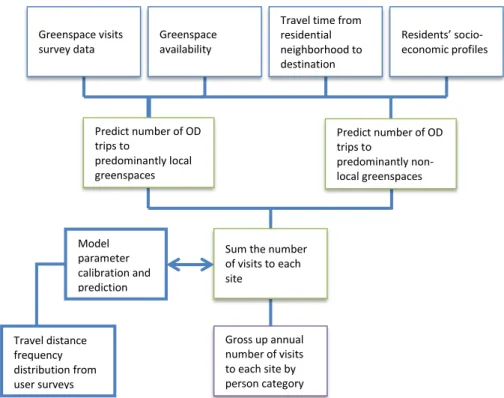
The trip generation function models a dependent variable defined as the expected number of visits from a given outset area to a given site. Individuals have been categorised into a given homogeneous population Q, we use socioeconomic groups (UK Census, 2011). Each option has an associated net utility for an individual. The utility can be represented by two components, 1) travel time, and 2) a random part. In the logit discrete choice model, the random part is assumed to be independently and identically distributed (IID) following the double exponential (Gumbel Type II extreme value) distribution (see Section 2.2). This random utility has then been weighted by the area of available greenspace within each destination. Together the function calculates the probability of an individual’s choice of a destination for an outdoor recreational purpose. To generate an estimate of the number of visits, it is then multiplied by the mean total of trips per person per year (data from Natural England, 2009- 2013) and the total population in each socioeconomic group (UK Census, 2011).
Figure 1. Schematic representation of the model methodology
Through initial analysis of observation data (Natural England, 2013), we categorised recreational trips into two major types (See Figure 2). The first group of trips are predominantly local trips which are generated for short visits at the destination. Those are mainly daily visits to green spaces nearby as day- to-day routine trips. The second group of trips are predominantly non-local trips.
Those trips are for long visits to destinations such as the countryside, coastal areas or other cities or towns away from home. They usually happen during weekends or holidays, where attributes of the destination are more important than distance. This assumption is based on the travel time budget theory (Makhtarian and Chen, 2004), which states “At the aggregate level, travel expenditures initially appear to have some stability. Similar travel time and money budgets may be found within a sub-population and in certain areas”. The method to define the local and non-local trips is based on a review of previous studies on how long people will spend on traveling in average. Eg. 1.1–1.3hrs per traveller per day (Zahavi and Ryan, 1980; Zahavi and Talvitie, 1980), about 430hrs per person per year (Hupkes, 1982), 50mins to 1.1hrs per person per day (Bieber et al., 1994), 1.1hrs per person per day (Schafer and Victor, 2000) or 1.3hrs per person per day (Vilhelmson, 1999). In conclusion, Travel Time for Local Trips (day trips) is likely to be less than 1.3hrs (78mins) per person.
Considering an 8min penalty for people to get into their cars, a trip’s travel time that is less than 35mins (about 40km driving) is defined as a “Local Trip”. In this paper, we have used 40km as a benchmark distance to separate local trips (distance equal or less than 40km) from non-local trips.
Greenspace visits
survey data Greenspace availability
Travel time from residential neighborhood to destination
Residents’ socio- economic profiles
Predict number of OD trips to
predominantly local greenspaces
Predict number of OD trips to
predominantly non- local greenspaces
Sum the number of visits to each site
Travel distance frequency distribution from user surveys
Model parameter calibration and prediction
Gross up annual number of visits to each site by person category
Figure 2. Greater Manchester outdoor recreational trips’ distance choice. X axis represents distance (m) and Y axis represents number of trips per year. Observation data from the MENE
(2013) survey, charts are drawn by the author.
The pattern of predominantly local trips gives similar results to Perino et al.
(2011) in terms of a steep distance decay profile in destination choices (See Figure 3). On the other hand, the analyses of predominantly non-local trips
0 5000 10000 15000 20000 25000 30000 35000
1 5 9 13 17 21 25 29 33 37 41 45 49 53 57 61 65 69 73 77 81 85 89 93 97 101
Group 2 - Predominantly non-local trips
AB C1 C2 DE Total
0 20000 40000 60000 80000 100000 120000
1 2 3 4 5 6 7 8 9 10 11 12 13 14 15 16 17 18 19 20 21 22 23 24
Group 1 - Predominantly local trips
AB C1 C2 DE Total
prove the assumption from Sen et al. (2013), that the longer distance visits are strongly affected by other variables such as the attributes of the greenspaces rather than distance.
Figure 3. Distance decay function of marginal value for a 10ha park. Source: Perino et al, 2011
Building on the above assumptions, we estimate the TGF using a discrete choice logit model through two parts:
𝑉𝑉𝑉𝑉𝑖𝑖𝑖𝑖𝑖𝑖= 𝑆𝑆𝑖𝑖𝑏𝑏∗ exp�−𝜆𝜆𝑖𝑖𝑡𝑡𝑖𝑖𝑖𝑖�
∑𝑚𝑚𝑖𝑖=0𝑆𝑆𝑖𝑖𝑏𝑏∗ exp�−𝜆𝜆𝑖𝑖𝑡𝑡𝑖𝑖𝑖𝑖�∗ 𝐴𝐴𝐴𝐴𝑖𝑖𝑖𝑖
𝑉𝑉𝑉𝑉𝑖𝑖𝑖𝑖𝑖𝑖= 𝑆𝑆𝑖𝑖𝑏𝑏′∗ exp�−𝜆𝜆𝑖𝑖′𝑡𝑡𝑖𝑖𝑖𝑖�
∑𝑚𝑚𝑖𝑖=0𝑆𝑆𝑖𝑖𝑏𝑏′∗ exp�−𝜆𝜆𝑖𝑖′𝑡𝑡𝑖𝑖𝑖𝑖�∗ 𝐴𝐴𝐴𝐴𝑖𝑖𝑖𝑖
VLijx denotes average number of local recreation trips per person per year from residential neighbourhood i to destination j, in socio-economic group x. VNijx
denotes the number of non-local recreation trips from the same origin to the same destination and for the same group of people. Sj is the size of greenspace within destination j and m is the total number of destinations. b and 𝜆𝜆 are parameters for local trips, b’ and λ𝑖𝑖 ’ for non-local trips. x indicates socioeconomic group x. tij denotes the travel time from residential neighbourhood i to destination j. Alix and Anix denotes the average total of predominantly local or non-local trips per person per year from neighbourhood i in socioeconomic group x.
N(j) = ∑ [∑ (V𝑉𝑉𝑘𝑘 𝑖𝑖𝑖𝑖𝑖𝑖 + VN𝑖𝑖𝑖𝑖𝑖𝑖) ∗ 𝑃𝑃𝐴𝐴𝑖𝑖𝑖𝑖 𝑟𝑟 𝑖𝑖=0
𝑖𝑖=0 ]
N(j) is the total annual number of visits at destination j. r represents the total number of socioeconomic groups. k is the total number of residential neighbourhoods i. Plix means the population of socioeconomic group x in residential neighbourhood i.
3.2 Data
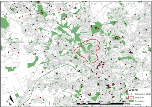
Observations of outdoor recreational visits were taken from the MENE 2009- 2013 survey (Natural England, 2013). It is a questionnaire based annual survey of how and why people engage with the natural environment. Individuals from selected households are interviewed for diary records of their recreational trips in the week running up to the interview date. One of these trips is then selected at random and the geographic location of the destination is recorded. The latest survey was carried out from March 2012 to February 2013. The observation data we used for calibration and validation purposes amounted to 2,900 interviews in the Great Manchester area, and more than 650 places have been identified.
Figure 4. Destinations from MENE survey data 2009-2013.
Figure 5. Population weighted LSOA centres.
Source: The UK Census, 2011.
Figure 6. Observed outdoor recreational trips distances for England, Greater Manchester and Salford.
Source: The MENE Annual Report, 2013.
36%
39%
41%
48%
40%
26%
26%
27%
26%
26%
17%
16%
15%
13%
15%
21%
19%
17%
14%
18%
0% 20% 40% 60% 80% 100%
AB C1 C2 DE ALL
England
36%
42%
54%
58%
47%
26%
23%
19%
20%
22%
17%
17%
11%
11%
15%
21%
18%
16%
11%
17%
0% 20% 40% 60% 80% 100%
AB C1 C2 DE All
Greater Manchester
7%
38%
44%
62%
42%
20%
26%
19%
17%
20%
25%
14%
16%
11%
16%
47%
22%
21%
10%
22%
0% 20% 40% 60% 80% 100%
AB C1 C2 DE ALL
Salford
Less than 1.6 km 1.6 or 3.2 km 4.8 to 8 km Over 8 km
approximately 16 km2and includes 40 Census Lower Super Output Areas. We have used the population weighted centres as the origins for trips. The MENE annual report (Natural England, 2013) indicates that more than 80% of people are willing to travel less than 8 km for outdoor recreational purposes. These patterns are consistent from the whole England scale to the Greater Manchester area. The pattern for the Salford area does not look very stable due to the very small sample size (162).
We expanded our research area by applying an 8 km radius buffer around each single origin, and defined the destination using 1km squares; the data in Figure 6 show more than 80% of adults travelled less than 5 miles (equal to 8 km) for outdoor recreational trips. There are two main criteria for identifying destinations: first is the location of the destination from the MENE survey and second is the availability of greenspace from the Open Street Map. Eighty-one destinations have been located within an 8 km radius buffer and their geometrical centres are later used for calculating travel time. We also create a 10km2 grid acting as a proxy for the other 20% of destinations more than 10km away.
Figure 7. 8km (5 mile) buffer, as the MENE survey suggests, 80% of the destinations for adults who live in the studying area should be drawn from within this buffer area.
Figure 8. Destinations defined by 1 km2 grids, drawn by the author.
Travel time from population weighted centroids of all LSOAs to destination sites were calculated using the OS Integrated Transport Network. This is a GIS dataset consisting of motorways, A-roads, B-roads, minor roads, pedestrian footpaths and cycle ways. Data from Jones et al. (2010) were employed to make allowances for varying average road speeds. The travel time calculated through the OD Matrix tool in ArcMap was validated by traveling times from Google Map.
Socioeconomic status has also made a significant difference on peoples’
behaviours regarding outdoor recreation trips (Sen et al., 2013, Natural England, 2013). We took account of variations by dividing the whole population into four different socioeconomic groups according to national census data.
Table 1. Socioeconomic status classification. Source: The UK Census, 2011.
Socioeconomic Group
AB Higher and intermediate
managerial/administrative/professional occupations C1 Supervisory, clerical and junior
managerial/administrative/professional occupations
C2 Skilled manual occupations
DE Semi-skilled and unskilled manual occupations; unemployed and lowest grade occupations
4. RESULTS
The estimations of models have been presented in Table 2, below. As expected, travel time plays a less important role for non-local destinations than for the local destinations. In contrast, as the area of a greenspace increases, so does the ratio of the number of trips from local and non-local destinations move to favour the non-local trips. Meanwhile, for both local and non-local destinations, travel time is more important to the people who are in the lower socioeconomic groups when making their travel decisions.
Socioeconomic Group Calibrated Model
Component a). Predominantly Local Trips
AB 𝑉𝑉𝑉𝑉𝑖𝑖𝑖𝑖{AB} = 𝑆𝑆𝑖𝑖0.2 ∗ exp�−0.56𝑡𝑡𝑖𝑖𝑖𝑖�
∑m𝑖𝑖=0𝑆𝑆𝑖𝑖0.2∗ exp�−0.56𝑡𝑡𝑖𝑖𝑖𝑖�∗ 47.73
C1 𝑉𝑉𝑉𝑉𝑖𝑖𝑖𝑖{C1} = 𝑆𝑆𝑖𝑖0.2 ∗ exp�−0.6𝑡𝑡𝑖𝑖𝑖𝑖�
∑m𝑖𝑖=0𝑆𝑆𝑖𝑖0.2∗ exp�−0.6𝑡𝑡𝑖𝑖𝑖𝑖�∗ 34.84
C2 𝑉𝑉𝑉𝑉𝑖𝑖𝑖𝑖{C2} = 𝑆𝑆𝑖𝑖0.2 ∗ exp�−0.72𝑡𝑡𝑖𝑖𝑖𝑖�
∑m𝑖𝑖=0𝑆𝑆𝑖𝑖0.2∗ exp�−0.72𝑡𝑡𝑖𝑖𝑖𝑖�∗ 34.31
DE 𝑉𝑉𝑉𝑉𝑖𝑖𝑖𝑖{DE} = 𝑆𝑆𝑖𝑖0.2 ∗ exp�−73𝑡𝑡𝑖𝑖𝑖𝑖�
∑m𝑖𝑖=0𝑆𝑆𝑖𝑖0.2∗ exp�−0.73𝑡𝑡𝑖𝑖𝑖𝑖�∗ 35.48
Component b). Predominantly Non-local Trips
AB 𝑉𝑉𝑉𝑉𝑖𝑖𝑖𝑖{AB} = S𝑖𝑖∗ exp(−0.001𝑡𝑡𝑖𝑖𝑖𝑖)
∑ Smj=0 𝑖𝑖∗ exp(−0.001𝑡𝑡𝑖𝑖𝑖𝑖)∗ 37.5
C1 𝑉𝑉𝑉𝑉𝑖𝑖𝑖𝑖{C1} = S𝑖𝑖∗ exp�−0.002𝑡𝑡𝑖𝑖𝑖𝑖�
∑ Smj=0 𝑖𝑖∗ exp�−0.002𝑡𝑡𝑖𝑖𝑖𝑖�∗ 21.35
C2 𝑉𝑉𝑉𝑉𝑖𝑖𝑖𝑖{C2} = S𝑖𝑖∗ exp�−0.006𝑡𝑡𝑖𝑖𝑖𝑖�
∑ Smj=0 𝑖𝑖∗ exp�−0.006𝑡𝑡𝑖𝑖𝑖𝑖�∗ 16.9
DE 𝑉𝑉𝑉𝑉𝑖𝑖𝑖𝑖{DE} = S𝑖𝑖∗ exp�−0.008𝑡𝑡𝑖𝑖𝑖𝑖�
∑ Smj=0 𝑖𝑖∗ exp�−0.008𝑡𝑡𝑖𝑖𝑖𝑖�∗ 11.83
The combined result was well validated with the observed MENE data, in a way that satisfies the standard requirements of travel demand prediction models.
Figure 9. Modelled outdoor recreational trips in the study area.
47%
36%
42%
54%
59%
28%
32%
30%
24%
24%
8%
11%
9%
7%
5%
16%
21%
18%
15%
11%
0% 20% 40% 60% 80% 100%
ALL AB C1 C2 DE
Salford (Modelled)
Less than 1.6 km 1.6 or 3.2 km 4.8 to 8 km Over 8 km
5. CONCLUSIONS AND FUTURE WORK
Our integrated model has two components for (a) predominantly local trips and (b) predominantly non-local trips. Unlike existing methods, both components of our model are based on the discrete choice model, which gives a transparent representation of the choices of greenspace sites visited. This is also more consistent with residents’ destination choice. When the model is used to test scenarios, it combines greenspace in urban and rural areas as a whole infrastructure instead of treating them separately. Component (a) gives similar results to Perino et al. (2011) in terms of a steep distance decay profile in destination choices, which is strongly influenced by travel time and socio- economic profiles, and relatively weakly by greenspace size. Component (b) gives similar results to Sen et al. (2013), with a gentle distance decay – the longer distance visits are strongly affected by greenspace size.
We have realized that greenspace size alone would not be able to describe all the attraction for visits. More detailing of attributes, such as the percentage of different types of land cover within each destination will be explored in the next stage of work. This may provide us with the answer to “what kind of greenspace will attract more visits?” This is a very hard question for urban green space modelling which has not been satisfactorily answered in the existing literature.
We hope we will be able to make significant progress in the next steps.
Meanwhile, the value of a single trip per person will also be reviewed based on existing literature. The ultimate objective of this study is to provide a toolkit which is able to quantify a greenspace’s recreational value.
One main challenge is to obtain detailed observations for validation; it is rare to find origin-destination surveys or even systematic arrivals for greenspace sites.
New social media data may have some potential in filling this gap. It would seem necessary to develop a new research agenda to collect such information in order to strengthen the empirical basis of the model.
Acknowledgements. Xihe Jiao wishes to acknowledge the funding support of a PhD Scholarship from the China Scholarship Council. All the maps are drawn based on data obtained at Edina, the Jisc-designated national data centre at the University of Edinburgh. Ying Jin wishes to acknowledge partial funding support of the Tranche 1 research grant funded by the EPSRC Centre for Smart Infrastructure and Construction at Cambridge University (EPSRC reference EP/K000314/1), and of the research grant from the Tsinghua-Cambridge-MIT Low Carbon Energy Alliance (Tsinghua University reference: TCMA2010). The usual disclaimers apply and the authors alone are responsible for any views expressed and any errors remaining.
REFERENCES
Andrews, B. (2009) “An investigation into the effects of distance and environmental attitudes on preferences for new parks in Norwich”, in: unpublished MRes dissertation, University of East Anglia, Norwich
Bateman, I. J., Harwood, A. R., Mace, G. M., Watson, R. T., Abson, D. J., Andrews, B. and Termansen, M. (2013). “Bringing ecosystem services into economic decision-making: land use in the United Kingdom”, Science, 341(6141), 45-50.
Bieber A, Massot M H, Orfeuil J P. Prospects for daily urban mobility. Transport Reviews, 1994, 14(4): 321-339.
CabeSpace (2005) “Does money grow on trees?”, CABE, London, 87pages
Davies, L., Batty, M., Beck, H., Brett, H., Gaston, K.J., Harris, J.A., Kwiatkowski, L., Sadler, J., Scholes, L., R.Sheate, W., Wade, R., Burgess, P., Cooper, N., McKay, H.I., Metcalfe , R.
and Winn, J. (2011), “Urban Broad Habitat”, UK National Ecosystem Assessment, Chapter 10
Dehring, C. and Dunse, N. (2006) “Housing density and the effect of proximity to public open space in Abderdeen”, Scotland, Real Estate Economics, 34(4), 553-566
Charles River Associates research study”, Economic analysis, (93).
Dunse, N., White. M. and Dehring, C. (2007) “Urban parks, open space and residential property values”, RICS Research paper series, 7(8) 40 pages
Hupkes G. The law of constant travel time and trip-rates. Futures, 1982, 14(1): 38-46.
Jones A., Wright J., Bateman I., and Schaafsma M. (2010), “Estimating arrival numbers for informal recreation: a geographical approach and case study of British woodlands”, Sustainability, 2:684–701
Millennium Ecosystem Assessment (2005), Ecosystems and Human Well-Being: Synthesis, Island Press, Washington, DC
Mokhtarian P L, Chen C. TTB or not TTB, that is the question: a review and analysis of the empirical literature on travel time (and money) budgets. Transportation Research Part A:
Policy and Practice, 2004, 38(9): 643-675.
Natural England (2013), “Monitor of Engagement with the Natural Environment: The national survey on people and the natural environment”. MENE Annual Report from the 2012-13 Survey, NECR122.
Office for National Statistics, 2011, Census: Digitised Boundary Data (England and Wales) Ortúzar, J. D., & Willumsen, L. (2011), “Discrete choice model”, Modelling Transport. 4th.
Perino, G., Andrews, B., Kontoleon, A., and Bateman, I. (2011). “Urban greenspace amenity- economic assessment of ecosystem services provided by UK urban habitats”. Report to the UK National Ecosystem Assessment, University of East Anglia, Norwich. [online]
Available at:< http://uknea. unep-wcmc.org/Resources/tabid/82/Default. aspx>[Accessed 23.03. 11].
Schafer A, Victor D G. The future mobility of the world population. Transportation Research Part A: Policy and Practice, 2000, 34(3): 171-205.
Sen, A., Harwood, A. R., Bateman, I. J., Munday, P., Crowe, A., Brander, L., and Provins, A.
(2014). “Economic assessment of the recreational value of ecosystems: Methodological development and national and local application”. Environmental and Resource Economics, 57(2), 233-249.
Spear, B. D. (1977). “Applications of new travel demand forecasting techniques to transportation planning”. A study of individual choice models (No. FHWA/PL-77012) Vilhelmson B. Daily mobility and the use of time for different activities. The case of Sweden.
GeoJournal, 1999, 48(3): 177-185.
Williams, H. C. (1977). “On the formation of travel demand models and economic evaluation measures of user benefit”. Environment and Planning A,9(3), 285-344.
Zahavi Y, Ryan J M. Stability of travel components over time. Transportation research record, 1980 (750).
Zahavi Y, Talvitie A.(1980). Regularities in travel time and money expenditures.