Dynamic Linear Hybrid Automata and Their Applications to Formal Verification of Dynamic Reconfigurable Embedded Systems

(1)

Dynamic Linear Hybrid Automata and Their

Applications to Formal Verification of Dynamic Reconfigurable Embedded Systems

著者柳瀬龍

著者別表示 Yanase Ryo journal or

publication title

博士論文要旨Abstract 学位授与番号 13301甲第4547号

学位名博士（工学）

学位授与年月日 2017‑03‑22

URL http://hdl.handle.net/2297/48034

Creative Commons : 表示 ‑ 非営利 ‑ 改変禁止

(2)

Abstract for Dissertation

Dynamic Linear Hybrid Automata and Their Applications to Formal Verification of Dynamic

Reconfigurable Embedded Systems

動的線形ハイブリッドオートマタと動的再構成可能組込みシステムの形式検証への応用

Ryo YANASE

(Student Number: 1323112012)

Graduate School of Natural Science and Technology Division of Electrical Engineering and Computer Science

Kanazawa University

Chief supervisor: Prof. Satoshi YAMANE

January 2017

(3)

Abstract

Networking systems and embedded systems are able to change their configuration, components and modules at run-time. Such a system is called dynamically reconfigurable system. For guaranteeing safety of the system, model checking is one of the eﬀective methods. This paper presents a dynamic linear hybrid automaton (DLHA) as a specification language for designing dynamically reconfigurable systems. As a practical experiment, we describe an embedded cooperative system consisting of CPU and DRP by DLHAs and verify several properties for the system with a model checker that performs the reachability analysis by using monitor automata.

1 Introduction

Dynamically reconfigurable systems are being used in a number of areas [1, 2, 3]. The major methods of checking system safety include simulation and testing; however, it is often diﬃcult for them to ensure safety precisely, since these methods don’t check all states. In such cases, model checking is a more eﬀective method. In this paper, we propose the Dynamic Linear Hybrid Automaton (DLHA) specification language for describing dynamically reconfigurable systems and provide a reachability analysis algorithm for verifying system safety.

1.1 Features of dynamically recon- figurable systems consisting of CPU and DRP

The target of our research is an embedded system in which a CPU and dynamically reconfigurable hardware, e.g., DRP or D-FPGA [4] operate co- operatively. The dynamically reconfigurable processor (DRP) is a coarse-grained programmable processor developed by NEC [3] and it manages both the power conservation and miniaturization.

The DRP is used to accelerate the computations of a general purpose CPU with through cooperating operations, and it has the following features:

• Dynamically creation/destruction of the function: when a process occurs, the DRP consti- tutes a private circuit for processing it. The

circuit configuration is released after the process finishes.

• Hybrid property: the operation frequency changes whenever a context switch occurs.

• Parallel execution: the DRP executes several processes on the same board at the same time.

• Queue for communication: the DRP asynchronously receives processing requests from the CPU.

For the experiments, we specified a dynamically reconfigurable embedded system consisting of a CPU and DRP, and verified the some of its im- portant features. This is the first time that specification and verification of dynamic changes have been tried in a practical case.

1.2 Related Work

1.2.1 Specification

We developed a new specification language (DLHA) based on a linear hybrid automaton [5]

with both creation/destruction events and unbounded FIFO queues. DLHA is diﬀerent from existing research in the following points:

• V. Varshavsky and others proposed the GALA (Globally Asynchronous - Locally Arbitrary) modeling approach including timed guards [6].

This approach cannot describe hybrid systems since it is the specification language based on discrete systems. Thus, GALA cannot repre- sent changes in operating frequency.

• S. Minami and others have specified a dynamically reconfigurable system using linear hybrid automata and have verified it by using a model checker, HYTECH[7]. Since linear hybrid automata cannot describe changes to the configuration and asynchronous communica- tions by using unbounded FIFO queues, the system has been specified as a static system.

• P. C. Attie and N. A. Lynch specified systems whose components are dynamically created/destroyed by using I/O automata [8].

I/O automata cannot describe changes in variables, for example, changes in clock and operating frequency.

(4)

• H. Yamada and others proposed hierarchical linear hybrid automata for specifying dynamically reconfigurable systems [9]. They intro- duced concepts such as class, object, etc., to the specification language. However, as the scale of a system to be specified increases, the representation and method of analysis in the verification stage tend to be complex.

• B. Boigelot and P. Godefroid specified a communication protocol in terms of finite- state machines and unbounded FIFO buﬀers (queues), and they verified it [10]. Since the finite-state machine also cannot describe changes in variables, it is unsuitable in our case.

• A. Bouajjani and others proposed a reachability analysis for pushdown automata and symbolic reachability analysis for FIFO-channel systems [11, 12]. However, since their analysis don’t provide for continuous changes in variables, in languages cannot be used for designing hybrid systems.

1.2.2 Verification Method

The originality of our work on the verification method twofold:

• Our method targets systems that dynamically change their configurations, which is some- thing the existing work, such as HYTECH, has studied. We extend the syntax and semantics of linear hybrid automata with special actions called creation actions and destruction actions. We define a state in which an au- tomaton does not exist and transitions for creation and destruction.

• Our method is a comprehensive symbolic verification for hybrid properties, FIFO queues and creation/destruction of tasks.

2 Dynamic Linear Hybrid Automaton

2.1 Syntax

A dynamic linear hybrid automaton (DLHA) is an extended linear hybrid automaton and represented

as a 8-tuple (L, V,Inv,Flow,Act, T, t0, Td), where

• L is a finite set of nodes called locations.

• V is a finite set of variables.

• Inv :L→Φ(V) is a function that assigns an invariant to each location, where Φ(V) is a set of all constraints overV.

• Flow:L→F(V) is a function that assigns a flow condition to each location, whereF(V) is a set of all flow conditions over V.

• Act =Actin∪Actout∪Actτ is a finite set of actions.

– Act_in is a finite set ofinput actions, and each input action has the forma?. An input actionm? denotes receiving the message m.

– Actout is a finite set of output actions, and each output action has the form a!.

An output action m! denotes broadcast- ing the messagemto each DLHA.

– Actτ is a finite set ofinternal actionsthat denote other events.

Moreover, we formalize the following special actions:

– A creation action that has the form Crt A^′? orCrtA^′! denotes a message for creation of the DLHA A^′. CrtA^′? is an input action, and it represents that A^′ has been created. CrtA^′!∈Act_out is an output action, and represents a request for creatingA^′.

– A destruction action that has the form Dst A^′? orCrtA^′! denotes a message for a destruction of DLHA A^′. DstA^′? ∈ Actinis an input action that indicatesA^′ has been destroyed.

– Anenqueue actionthat has the formq!m denotes enqueueing of message m into a queue q. This action is an internal one, that is,q!m∈Actτ.

– Adequeue actionthat has the formq?m denotes dequeueing of message m from the top of queueq.

(5)

• T ⊆L×Φ(V)×Act×2^UPD(V⁾×Lis a finite set of edges calledtransitions. Here, a constraint ϕ∈Φ(V) is called aguard condition, andλ∈ 2^UPD(V⁾ are called update expressions. Each update expression has the formx:=corx:=

x+c, where x∈V andc∈Q.

• t₀∈L×(Act_in∪Act_τ)×2^UPD(V⁾is aninitial transition.

• Td ⊆ L ×Φ(V)×Actout is a finite set of destruction-transitions.

2.2 Operational Semantics

A state σ of a DLHA (L, V,Inv,Flow, A, T, t0, Td) is defined as ⊥ | (l, ν), where l ∈ L is a location, ν : V → R is an assignment called evaluation of variables, and⊥denotes anundefined value.

The semantics M of the DLHA is defined as (Σ,⇒, σ0), where Σ is a set of states,⇒is a set of time transitions anddiscrete transitions andσ0 is the initial state.

2.2.1 Time transition For arbitrary δ∈R≥0,

• ⊥⇒δ⊥,

• (l, ν)⇒δ(l, ν^′) ifν^′ =ν+δ·Flow(l)∈Inv(l), whereν^′ =ν+δ·Flow(l) denotes an evaluation such that∀x∈V.ν^′(x) =ν(x)+δ·x˙·Flow(l)(x), andν^′ ∈ Inv(l) denotes that ν^′(x) satisfies the constraint Inv(l) for anyx∈V.

2.2.2 Discrete transition

For an evaluation ν and update expressions λ ∈ 2^UPD(V⁾,ν[λ] denotes an evaluation updated byλ.

• For any transition (l, ϕ, a, λ, l^′)∈T, (l, ν)⇒a

(l, ν[λ]) ifν ∈ϕandν[λ]∈Inv(l^′).

• (Creation of a DLHA) For the initial transi- tiont₀= (l₀, a₀, λ₀),⊥⇒a0 (l₀, ⃗0[λ₀]) where⃗0 is an evaluation such that∀x∈V.[⃗0(x) = 0].

• (Destruction of a DLHA) For any destruction- transition

(l, ϕ, a)∈Td, (l, ν)⇒a⊥ifν∈ϕ

For the initial transition (l0, a0, λ0), the initial stateσ0is defined as

σ₀=

{⊥ (a0∈Actin) (l0, ⃗0[λ0]) (otherwise).

3 Dynamically Reconfig- urable Systems

To describe an asynchronous communication among DLHAs in a dynamically reconfigurable system, we use a queue (unboundedFIFO buﬀer) as a model of the communication channel. We assume that the system performs lossless transmission, so we can let the queue be unbounded.

A dynamically reconfigurable systemS= (A,Q) consists of a finite setA={A1, . . . ,A_|A|} of DL- HAs and a finite setQ={q₁, . . . , q_|Q|} of queues.

A statesof the dynamically reconfigurable system is a tuple⟨⃗σ, ⃗w_Q⟩where⃗σis a vector of states of DLHAs andw⃗_Qis a vector of contents of queues.

3.0.1 Time Transition

For an arbitrary δ ∈ R_≥0, the time transition is defined as

⟨⃗σ, ⃗w_Q⟩ →δ ⟨⃗σ^′, ⃗w_Q⟩ ⇐⇒ ∀i.σ_i⇒δσ_i.

3.0.2 Discrete Transition

Let⃗σ, ⃗σ^′, ⃗w_Q and w⃗^′_Q be ⃗σ = (σ1, . . . , σ_|_A_|), ⃗σ^′ = (σ^′₁, . . . , σ_|^′_A_|), w⃗_Q = (w1, . . . , w_|Q|) and w⃗_Q^′ = (w^′₁, . . . , w^′_|Q|).

• For any output actiona!,⟨⃗σ, ⃗w_Q⟩ →a⟨⃗σ^′, ⃗w_Q⟩ iﬀ∃i.σi⇒a!σ_i^′∧ ∀j̸=i.σj ⇒a?σj

∨((¬∃σ_j^′.σj⇒a?σ^′_j)∧σj =σ^′_j).

An output action is broadcasted to all DL- HAs, and a DLHA receiving the action moves by synchronization if the the guard condition holds in the state.

• For an internal actionaτ,

– in the case of aτ =qk!w, ⟨⃗σ, ⃗w_Q⟩ →q_k!w

⟨⃗σ^′, ⃗w^′_Q⟩,

iﬀ∃i.σ_i⇒qk!wσ_i^′∧ ∀j̸=i.σ_j=σ_j^′

∧w_k^′ =wkw∧ ∀l̸=k.wk =w_k^′,

(6)

– while in the case of aτ = qk?w,

⟨⃗σ, ⃗w_Q⟩ →q_k?w⟨⃗σ^′, ⃗w^′_Q⟩,

iﬀ∃i.σi⇒q_k?wσ_i^′∧ ∀j̸=i.σj=σ_j^′

∧w_k =ww_k^′ ∧ ∀l̸=k.w_l=w_l^′, – otherwise, ⟨⃗σ, ⃗w_Q⟩ →aτ ⟨⃗σ^′, ⃗w_Q⟩,

iﬀ∃i.σ_i⇒aτ σ^′_i∧ ∀j̸=i.σ_j =σ_j^′. Arun (or path)ρof the systemSis the following finite (or infinite) sequence of states.

ρ: s₀→^δa⁰₀ s₁→^δa¹₁ · · · →^δ^aⁱ⁻¹i−1 s_i→^δaⁱ_i · · · where →^δaⁱ_i between si and si+1 is defined as follows:

si →^δaⁱi si+1 ⇐⇒ ∃s^′_i.si→δ_i s^′_i∧s^′_i→a_i si+1. The initial state s0 is a tuple

⟨(σ₀₁. . . , σ0|A|),(w₀₁, . . . , w0|Q|)⟩, where each σ0i is the initial state of DLHA Ai and eachw0j

is empty; that is, ∀j.w0j=ε.

4 Reachability Analysis

4.1 Reachability Problem

We define reachability and the reachability problem for a dynamically reconfigurable system as follows:

Definition 1 (Reachability) For a dynamically reconfigurable systemS= (A,Q)and a locationlt, S reachesltif there exists a paths0→^δa⁰0 · · · →^δa^t−1_t−1

st such that st has a DLHA-state which contains the locationlt.

Definition 2 (Reachability Problem) Given a dynamically reconfigurable system S = (A,Q) and a location lt, we output “yes” if S can reach lt, and “no” otherwise.

4.2 Algorithm of Reachability Anal- ysis

Fig. 1 show the algorithm of the reachability analysis. Our method introducesconvex polyhedra for the reachability analysis in accordance with [17].

In this algorithm, we define a statesin the reachability analysis as (L, ζ, ⃗w_Q), whereLis a finite set

of locations,ζis a convex polyhedron, andw⃗_Qis a vector of contents of queues. Fig.1 is an overview of the reachability analysis, and this algorithm is performed by using the extended method of [13]

with a setQ of queues. The analysis is performed as follows:

1. Compute the initial state s0 of the system S (ll.1–3).

2. Initialize a traversed set Visit and a untra- versed set Wait of states by∅and {s0} (line 4).

3. While Wait is not empty, repeat the following process (ll.5–16).

(a) Take a state (L, ζ, ⃗w_Q) from Wait and remove the state from Wait (ll.6–7).

(b) If the setLof locations contains the target location, return “yes” and terminate (ll.8–10).

(c) If the state has not been traversed yet ((L, ζ, ⃗w_Q)̸∈Visit) (line 11),

i. add the state to Visit (line 12), ii. compute the set S_post of successors

by using the subroutine Succ (line 13), and

iii. add all components ofSpost to Wait (line 14).

The subroutine Succ computes successors of a state. Successors for a statestogether with a transition that has an output action are computed by the following procedures:

1. InitializeSpost by∅.

2. Compute a convex polyhedron ζδ for time transition.

3. For eachAi in the systemS, compute the set T_si of transitions that are outgoing from the state by using the input actional?.

4. Compute a set ∆ of combinations ofT_si. 5. For each combination T = (t₁, . . . , t_n) ∈ ∆,

the successor s^′ = (L^′_T, ζ_T^′, ⃗w_Q) is computed andS_post:=S_post∪ {s^′}.

The correctness of this algorithm is implied by Lemma 1 and Lemma 2.

(7)

Lemma 1 If this algorithm terminates and re- turns “lt is not reachable”, the system S holds the safety property.

Lemma 2 If this algorithm terminates and re- turns “lt is reachable”, the systemS does not hold the safety property.

By definition, all linear hybrid automata are DL- HAs. Our system dynamically changes its structure by sending and receiving messages. However, the messages statically determine the structure, and the system is a linear hybrid automaton with a set of queues. It is basically equivalent to the reachability analysis of a linear hybrid automaton.

Therefore, the reachability problem of dynamically reconfigurable systems is undecidable, and this algorithm might not terminate [13].

Moreover, in some cases, a system will run into an abnormal state in which the length of a queue becomes infinitely long, and the verification proce- dure does not terminate.

Input: a systemS and a target locationlt

Output: “yes” or “no”

1: L0← {l0i |t0i= (l0i, a0i, λ0i), a0i̸=CrtAi?}

2: λ0 ← ∪

{λ0i | t0i = (l0i, a0i, λ0i), a0i ̸= CrtAi?}

3: s0←(L0, ⃗0[λ0],(ε, . . . , ε)) /* Compute the initial state */

4: Visit←∅,Wait← {s₀} /* Initialize */

5: whileWait̸=∅do

6: (L, ζ, ⃗w_Q)←s∈Wait

7: Wait←Wait\ {(L, ζ, ⃗w_Q)}

8: if lt∈Lthen

9: return “yes”

10: end if

11: if (L, ζ, ⃗w_Q)̸∈Visit then

12: Visit←Visit∪ {(L, ζ, ⃗w_Q)}

13: Spost ← Succ((L, ζ, ⃗w_Q),S) /* Compute the set of post-states */

14: Wait←Wait∪Spost 15: end if

16: end while

17: return “no”

Figure 1: Reachability Analysis

5 Practical Experiment

5.1 Model Checker

We implemented a model checker of dynamically reconfigurable systems consisting of DLHAs in Java (about 1,600 lines of code) by using the LAS, PPL, and QDD external libraries [10, 14, 15, 16].

For the verification, we input the DLHAs of the system, a monitor automaton, and the error lo- cation to the model checker, and it output “yes (reachable)” or “no (unreachable)”. The monitor automaton had a special location (we call it the error location), and checked the system without changing the system’s behavior [17]. The monitor automata had to be specified to reach the error location if the system didn’t satisfy the properties.

For the specification of the input model, we extended the syntax and semantics of DLHA as follows:

• A transition between locations can have a la- bel asap (that means ‘as soon as possible’).

For a transition labeled asap, a time transi- tion does not occur just before the discrete transition.

• Each DLHA can have constraints and update expressions for the variables of another DLHA in the same system. That is, for each DLHA, invariants, guard conditions, update expressions and flow conditions can be used by all DLHAs.

5.2 Specification of Dynamically Reconfigurable Embedded Sys- tem

5.2.1 A cooperative system including CPU and DRP

We have specified a dynamically reconfigurable embedded system consisting of a CPU and DRP for the model described in our previous research [7].

A DRP has computation resources calledtiles (or processing elements), and it dynamically sets the context of a process if there are enough free tiles.

In addition, a DRP can change the operating frequency in accordance with running processes. In this paper, we assume that the number of tiles and the operating frequency for each process have been

(8)

set in advance and that the operating frequency of the DRP is always the minimum frequency of the running co-tasks.

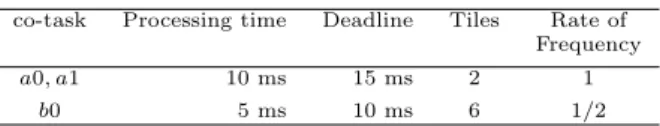
Fig. 2 shows an overview of the system. This system processes jobs submitted from the external environment through the cooperative operation of the CPU and DRP. The CPU Dispatcher creates a task when it receives a call message of the task from the external environment. When a task on the CPU uses the DRP, The CPU Dispatcher sends a message to the DRP Dispatcher. The DRP Dis- patcher receives the message asynchronously and creates aco-task(it means ‘cooperative task’) in a first-come, first-served manner if there are enough free tiles. Here, we will assume that this system has two tasks and two co-tasks that have the parameters shown in Table 1-2.

Task A CPU Dispatcher

Task B

Co-task a DRP Dispatcher

Co-task a External Environment

CPU DRP

Cooperation

Tile

Co-task b

Figure 2: Overview of the CPU-DRP embedded system

EnvA EnvB

Scheduler

TaskA

DRP_Dispatcher

cotask_a0 cotask_a1 Frequency_

Manager

cotask_b0 TaskB

Environment

CPU DRP

Queue q Sender

Message Creation

Figure 3: Components of the system

The system, whose components are illustrated in Fig.3, consists of 11 DLHAs and 1 queue. The

Table 1: Parameters of tasks

Task Period Deadline Priority Process

A 70 ms 70 ms high 20 ms, co-task a0, 10 ms, co-task b0 B 200 ms 200 ms low co-task a1, 97 ms

Table 2: Parameters of co-tasks

co-task Processing time Deadline Tiles Rate of Frequency

a0, a1 10 ms 15 ms 2 1

b0 5 ms 10 ms 6 1/2

external environment consists of EnvA and EnvB that periodically create TaskA and TaskB. That is, EnvA creates TaskA every 70 milliseconds, and EnvB creates TaskB with every 200 milliseconds.

The Scheduler performs scheduling in accordance with the priority and actions for creation and destruction of DLHAs.

TaskA and TaskB send a message to The Sender if they need a co-task. The Sender enqueues the message to create a co-task toqwhen it receives a message from tasks.

The DRP Dispatcher dequeues a message and creates cotask a0, cotask a1, and cotask b0 if there are enough free tiles. The Frequency Manager is a module that manages the operating frequency of the DRP. When a DLHA of a co-task is created, The Frequency Manager moves to the location that sets the frequency to the minimum value.

5.2.2 Other cases

We have the parameters of the model in subsection 5.2.1 and conducted experiments with it.

• Modified Tasks: We modified the parameters of the tasks on the CPU as shown in Table 3.

Here, the parameters of the co-tasks are the same as those in Table 2.

• Modified co-tasks: We modified the parameters of the co-tasks on the DRP, as shown in Table 4. Parameters of the tasks are the same as those in Table 1.

(9)

Table 3: Modified parameters of tasks

Task Period Deadline Priority Process

A 90 ms 80 ms high 20 ms, co-task b0, 20 ms, co-task a0 B 200 ms 150 ms low co-task a1, 70 ms

Table 4: Modified parameters of co-tasks

co-task Processing time Deadline Tiles Rate of Frequency

a0, a1 5 ms 10 ms 4 1

b0 10 ms 20 ms 5 1/3

5.3 Verification Experiment

We verified that the embedded systems described in subsection 5.2 provide the following properties by using monitor automata. The verification experiment was performed on a machine with an Intel (R) Core (TM) i7-3770 (3.40GHz) CPU and 16GB RAM running Gentoo Linux (3.10.25-gentoo).

Verification properties are below:

• Schedulability: Here, schedulability is a property in which each task of the system finishes before its deadline. Let EA be the total processing time andDAbe the deadline in task A;

the remaining processing time is represented as EA−eA, and the remaining time till the deadline is represented as DA −rA. There- fore, the monitor automaton moves the error location if the task A is created and it satisfies the conditionE_A−e_A> D_A−r_A (Fig. 4).

• Creation of co-tasks: In the embedded system, each co-task must be created before the remaining time in the task calling it reaches its deadline. When the message create a0 is received from task A, the monitor automaton starts counting time for co-task a0. If the waiting time exceeds the deadline of task A before it receives the message Crt cotask a0, the monitor moves to error location.

• Destruction of co-tasks: Each co-task must be destroyed before the waiting time reaches its deadline. For the co-task a0, when the message Crt cotask a0 is received from the

dispatcher DRP Dispatcher, the monitor automaton checks the message Dst cotask a0.

• Frequency management: Creating or destroy- ing a co-task, the DRP changes the operating frequency corresponding to the co-tasks being processed. Since this system requires that the frequency is always at the minimum value, the monitor checks whether the frequency manager (Frequency Manager) moves to the cor- rect location when it receives a message for creating a co-task. For example, when co- task a0 and co-task b0 are running on the DRP, Frequency Manager must be at location L Freq b.

• Tile Management: When the DRP receives a message for creating of a co-task and the number of free tiles is enough to process it, the dispatcher creates the co-task. The dispatcher then updates the number of used tiles. The monitor automaton checks whether the num- bertilesin DRP Dispatcher is always between 0 and the maximum number, 8 in this case.

Figure 4: Monitor automaton checking schedulability

The experimental results shown in Table 5 indi- cate that the modified tasks cases and the modified

(10)

co-tasks cases were verified with less computation resources (memory and time) than were used by the original model. This reduction is likely due to the following reasons:

• Regarding the schedulability of the modified tasks model, the processing time is shorter than that of the original model since the verification terminates if a counterexample is found.

• In the cases of the modified co-tasks, the most obvious explanation is that the state-space is smaller than that of the original model since the number of branches in the search tree (i.e.

nondeterministic transitions in this system) is reduced by changing the start timings of the tasks and co-tasks with the parameters.

• In cases other than those of the modified tasks, it is considered that the state-space is smaller than that of the original model because this system is designed to stop processing when a task exceeds its deadline.

6 Conclusion and future work

In this paper, we proposed a dynamic linear hybrid automaton (DLHA) as a specification language for dynamically reconfigurable systems. We also devised an algorithm for reachability analysis and developed a model checker for verifying the system. Our future research will focus on a more eﬀective method of verification, for example, model checking with CEGAR (Counterexample- guided abstraction refinement) and bounded model checking based on SMT (Satisfiability modulo theories) [18, 19].

References

[1] P. Garcia, K. Compton, M. Schulte, E. Blem and W. Fu. An Overview of Reconfigurable Hardware in Embedded Systems. EURASIP J. Embedded Syst., 2006(1):1–19, 2002.

[2] J. W. Lockwood, J. Moscola, M. Kulig, D. Reddick and T. Brooks. Internet Worm and Virus Protection in Dynami- cally Reconfigurable Hardware. In Military

and Aerospace Programmable Logic Device (MAPLD), E10, 2003.

[3] M. Motomura, T. Fujii, K. Furuta, K. Anjo, Y. Yabe, K. Togawa, J. Yamada, Y. Izawa and R. Sasaki. New Generation Micropro- cessor Architecture (2):Dynamically Recon- figurable Processor (DRP). IPSJ Magazine, 46(11):1259–1265, 2005.

[4] H. Amano, Y. Adachi, S. Tsutsumi and K. Ishikawa. A context dependent clock control mechanism for dynamically reconfigurable processors. Technical Report of IEICE, 104(589):13–16, 2005.

[5] R. Alur, C. Courcoubetis, T. A. Henzinger and P. Ho. Hybrid automata: An algorithmic approach to the specification and verification of hybrid systems.Lecture Notes in Computer Science, 736:209–229, 1993.

[6] V. Varshavsky and V. Marakhovsky. GALA (Globally Asynchronous – Locally Arbitrary) Design. Lecture Notes in Computer Science, 2549:61–107, 2002.

[7] S. Minami, S. Takinai, S. Sekoguchi, Y. Nakai and S. Yamane. Modeling, Specification and Model checking of dynamically reconfigurable processors. Computer Software, 28(1):190–

216, 2011.

[8] P. C. Attie and N. A. Lynch. Dynamic input/output automata, a formal model for dynamic systems. Proceedings of the twenti- eth annual ACM symposium on Principles of distributed computing (PODC ’01), 2154:314–

316, 2001.

[9] H. Yamada, Y. Nakai and S. Yamane. Pro- posal of Specification Language and Verifi- cation Experiment for Dynamically Recon- figurable System. Journal of Information Processing Society of Japan, Programming, 6(3):1–19, 2013.

[10] B. Boigelot and P. Godefroid. Symbolic Verifi- cation of Communication Protocols with Infi- nite StateSpaces using QDDs.Form. Methods Syst. Des., 14(3):237–255, 1999.

(11)

Table 5: Experimental results

Model Property Satisfiability Memory [MB] Time [sec] States

Original: Schedulability yes 168 180 1220

Creation of co-tasks yes 92 315 1220

Destruction of co-tasks yes 154 233 1220

Frequency Management yes 173 265 1220

Tile Management yes 167 234 1220

Modified tasks: Schedulability no 105 10.2 91

Modified co-tasks: Schedulability yes 83 141 768

[11] A. Bouajjani, J. Esparza and O. Maler.

Reachability Analysis of Pushdown Au- tomata: Application to Model Checking. Lec- ture Notes in Computer Science, 1243:135–

150, 1997.

[12] A. Bouajjani and P. Habermehl. Symbolic reachability analysis of FIFO-channel systems with nonregular sets of configurations. Lec- ture Notes in Computer Science,1256:560–

570, 1997.

[13] R. Alur, C. Courcoubetis, N. Halbwachs, T. A. Henzinger, P. Ho, X. Nicollin, A. Oliv- ero, J. Sifakis and S. Yovine. The algorithmic analysis of hybrid systems. Theoretical Com- puter Science, 138:3–34, 1995.

[14] Y. Ono and S. Yamane. Computation of quan- tifier elimination of linear inequlities of first order predicate logic. IEICE Technical Re- port. COMP, Computation, 111(20): 55–59, 2011.

[15] R. Bagnara, P. M. Hill and E. Zaﬀanella. The Parma Polyhedra Library: Toward a complete set of numerical abstractions for the analysis and verification of hardware and software systems. Sci. Comput. Program., 72(1–2): 3–21, 2008.

[16] B. Boigelot, P. Godefroid, B. Willems and P. Wolper. The Power of QDDs (Extended Abstract). SAS, 172-186, 1997.

[17] T. A. Henzinger, P. Ho and H. Wong-toi.

HyTech : A Model Checker for Hybrid Sys- tems.Software Tools for Technology Transfer, 1: 460–463, 1997.

[18] E. M. Clarke, O. Grumberg, S. Jha, Y. Lu and H. Veith. Counterexample-Guided Ab- straction Refinement. Proceedings of the 12th International Conference on Computer Aided Verification, 1855:154–169, 2000.

[19] R. Nieuwenhuis, A. Oliveras and C. Tinelli.

Abstract DPLL and abstract DPLL modulo theories. In LPAR 04, LNAI 3452, 36–50, 2005.

(12)