SOME IMPORTANT PROPERTIES OF
HIGH-ORDER FINITE-DIFFERENCE SCHEMES FOR LAPLACE EQUATrONI
by Xiping Yu2
An inherent contradiction in the finite-difference methods for the Laplace equation is demonstrated.
The grid size in a practical computation must, on the one hand, be fine enough to ensure the numerical accuracy, but, on the other hand, be necessarily large to avoid an ill-conditioned difference equation system, Higher-order schemes are shown to be advantageous in terms of both the accuracy and the condition of the difference equation system.
where aH, av and (J are coefficients depending on the shape of the grid element.
Typical Schemes
Consider the Laplace equation:
We assume that the finite-difference scheme of interest is in general a nine-point one and corre- lates the values of the independent variable at the nine nodes of the rectangular grid element (Fig. 1) in the following manner:
(2)
(1)
ePo=aH(ePEC+ePwc)+aveePNC+ePsc)
+/3( ePNE+ePSE+ePNW+ePsw)
It is well understood that the accuracy is an important but not the only criterion in evaluating a finite-difference scheme. Among the other impor- tant items for schemes of elliptic partial differen- tial equations is the condition of the finite-differ- ence equation system resulted from the application of the relevant scheme. In the present study, we examine some important properties of high-order schemes of the Laplace equation. Emphasis is paid on an inherent contradiction in pursuing a not only accurate but also well-conditioned scheme.
Introduction
Development of high-order schemes for the La- place equation has been very active. The "best"
nine-point scheme for square grid elements, of the eighth-order accuracy, was obtained by Bickley (1948), Greenspan (1957), Kantorovich and Krylov (1958) and Fox (1962). Derivation of the relevant scheme for rectangular grid elements with arbi- trary width-to-Iength ratio has also been paid attention since 1980s. Manohar and Stepheson (1982) presented a scheme of the sixth-order by assuming that the local solution of the Laplace equation can be approximated by a polynomial of degree four in both independent variables. To avoid the negative coefficients in Manohar and Stepheson's (1982) scheme that arise when the width- to-length ratio of grid element is large, Chwang and Chen (1987) proposed the "optimal"
scheme, which is essentially identical to Manohar and Stepheson's (1982) scheme but adopts a lower- order algorithm as the width-to-Iength ratio of the grid elements becomes relatively large or small.
With a rather different approach, Chen et al. (1980) obtained the so-called finite-analytic scheme.
The finite-analytic scheme seems to be equivalent to a fourth-order scheme in general, but its coeffi- cients are always positive.
1 Received on October 16, 1995
2 Department of Civil Engineering
y
NW Ee NE
Ay
WC 0 EC
Ax
sw SC SW
Fig. 1 Definition sketch of a grid element.
Fig. 3 demonstrates the variation of aH, av and /3 for the finite-analytic scheme versus r. aH is shown to increase while av decrease asr increases;
/3, however, has a peak value at r=l.
The "best" nine-point scheme with the sixth- x order accuracy in general is represented by the
following coefficients:
10r2-2 (9)
aH 20+Z0r2
10-2r2 (10)
av ZO+ZOr2
1 (11)
/3=20
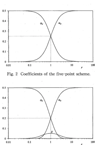
The five-point scheme (Lapidus and Pinder 1982) is probably the most classical finite-difference scheme for the Laplace equation. When represent- ed by (2), this scheme possesses thefollowing~coeffi
cients:
r 2 (3)
aH= 2+2r2
1 (4)
aV=2+2r2
/3=0 (5)
At r=l, aH=av=0.2 and /3=0.05. Variation of aH, avand /3 for the "best" scheme versus r is shown in Fig. 4. It is noticed that the scheme has the numer- ically unpopular negative coefficients at relatively large or small values of r (r>/5 or r<1//5).
This seems to be the cost of the possibly highest- order accuracy.
. Itshould be pointed out that the above schemes for the Laplace equation all satisfies the following
At r=l, aH=av=0.199Z684 and /3=0.0507316.
These values are very close to those of the "best"
nine-point scheme mentioned in the following.
where r=b..y/b..x is the width-to-Iength ratio of grid elements. Since /3 vanishes, the scheme involves only five nodes of the grid element.
Variation of aH and av of the five-point scheme versus r is demonstrated in Fig. 2. aH increases while av decreases as r increases. At r = 1, that is, for square grid, aH=av=1/4.
Chen et al. (1980) showed that the finite-analytic method can also be employed to derive a finite,-- difference scheme for the Laplace equation. Fol- lowing Chwang and Chen. (1987), the coefficients of the. finite-analytic scheme read
r 0.5
0.4
0.3
0.2
0.1
0
0.01 0.1 10 100
0.5
0.4
0.3
0.2
0.1
0
0.01 0.1 10 100
r
Fig. 3 Coefficients of the finite-analytic scheme.
Fig. Z Coefficients of the five-point scheme.
(6)
(8)
(7)
1 Jr
aH=Zsechzr
1 Jrr
av=zsech2
1 ( Jr Jrr)
/3=- I-sech --sech -
4 Zr Z
1 C(
C( 1 C(
0.5 A=
0.4~ a 1 a
0.3 a 1 (N-I)x(N-I)
0.2 a /3
(3 a (3
0.1
E==
/3 C( /3
(15)
(16)
(3 C( (N-I)X(N-I) 100
10 0.1
-0.1 -+---.--,-,...,...,.","",=---,..--,--,-Cj~_----r''''-r-,...,...,.:;:;:rr-...,,...,...,...,.,..,..
0.01 r
Fig. 4 Coefficients of the "best" nine-point scheme. The unknown vector relation:
This implies that the value of the dependent vari- able at the central node of a .grid element. is a weighted average of its values at the ambient nodes. This seems to be a necessary condition of any scheme for the Laplace equation, because any constant should be automatically a solution.
Condition' of Finite-Difference Equation System
Consider the finite-difference solution of a Diri- chlet problem defined over a a x a square domain.
We discretize the domain into square grid elements with b.x=b.Y=1/a, where 1/=I/N and N (d:2) is an integer. For square grid, we denote aH=aV=a.
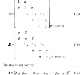
Application of a particular scheme at each inner node of the domain then gives rise to the following difference equation system:
b={bl,1 bl,z ... bl,N-I bZ,1 ... bN-I,N-I}T (18)
(19)
(20)
Ji._ltilmax - Itilm1n
A ¢ = . 1 ¢
is formed by the nodal values of the dependent variable and the right hand side vector
is determined by the boundary condition of the problem.
Whether matrix A is ill-conditioned can be deter- mined by the condition numberJi.,which, for a real and symmetric matrix, is expressed by (Young and Gregory 1988) :
where 1.1lmaxand1.1lmlnare the eigenvalues of A with maximum and minimum absolute values, respec- tively. When Ji. is very large, the matrix A and, consequently, the finite-difference method is il1- conditi oned.
Itis known that any eigenvalue of A, denoted by A, satisfies
(12)
A~=b (13) where
where
A S
E A E ¢ ={Ihi 1hz .•. IhNd r/JZ,I .,. r/JN-I,N-rY (21)
A=
E A E
E A (N-l)x(N-I)
(14) is the eigenvector of A corresponding to .1. Obvi- ously, (20) is equivalent to the following difference equation
is a tri-diagonal block matrix with each block expressed by one of the following exact tri-diago- nal matrices:
r/Ji,j - a(r/Ji-I,j+r/Ji+l,j+r/Ji,j-I+r/Ji,j+I)
- (3(Ij;;-I,J-I+r/Ji-I,j+l+r/Ji+I,J-I+r/Ji+l,J+l)
= .1r/Ji,j (22)
(i, j=l, 2, "',N -1)
with ¢O,j=¢N,j=(/;;'O=¢i,N=O. The solution of ¢ and Il can then be represented by
Illlmax=Il(N-l),{N-l) = 1+-..£cosJrl/_lCOS 2 Jrl/ (32)
5 5
¢T,f=sinim7wsinjmfl/
Ilm,n= 1- 2a(cosm7fl/+ cosmfl/)
- 4/3 cosmJrl/cosnJrl/
(m, n=l, 2, "', N -1)
(23)
(24)
Hence,
5 + 4 cos Jrl/ - cos2Jr1) f.L 5- 4 cos Jr1) - cos2JrV
(33)
(34) When the five-point scheme is applied, we have a
=1/4 and /3=0. (24) then becomes
For very fine grid,
(35)
(36)
¢=e- rrxcosJry
Similar to the five-point scheme, the "best" nine- point scheme is also ill-conditioned if the grid adopted is fine, and refining the grid leads to worse condition of the difference equation system. This property of the finite-difference equation system seems to be an inherent contradiction in the appli- cation of finite-difference method to the Laplace equation. On the one hand, the grid should be fine enough so that the truncation error of the scheme can be controlled. On the other hand, the grid should not be so fine so the system of the difference equation becomes ill-conditioned.
Comparing (35) with (30) we find that the condi- tion number of the "best" nine-point scheme is only 2/3 of that of the five-point scheme when the grid is fine. This simply means that the "best" nine- point scheme is advantageous in terms of not only the accuracy but also the condition of the finite- difference equation system.
Numerical Performance
To examine the behavior of various finite-differ- ence schemes for the Laplace equation, we apply them to the computation of a Dirichlet problem.
The domain of the problem is the interior region bounded by x=O, y=O, x=1 and y=1. The bound- ary condition of the problem is given in accordance to
(25)
(26) (27)
(28)
(30) (29) 1+ cos 7fl/
I-cos Jrl/
f.L~ Jr2l/24 ~00
\lllmax=NN-l),(N-I)=1+ cosJr1)
Illlmln=1l1,l=l-cos Jrl/
(28) leads to Therefore,
For very fine grid, i.e., at
This implies that all the eigenvalues of A are positive. Recalling that 1/N~ml/,nl/~1-1/N, we readily find
-51 cosmJr1)cos nJrl/
This means that the five-point finite-difference scheme is ill-conditioned if the grid adopted is fine.
We should also note that the finer the grid, the worse the condition of the difference equation sys- tem.
Now behold the "best" nine-point scheme. For square grid, a=I/5 and /3=1/20. (24), therefore, can be written as
Again, we note thatIlm,n are positive for all possible values ofm and n. Itcan also be shown, from (31), that
Since ¢ satisfies the Laplace equation and the solution of a Dirichlet problem of the Laplace equation is unique, (36) must also express the ana- lytic solution of the relevant problem. For numeri- cal solutions, the domain is discretized into square
10' j
E 10-1
10-2
10-3
10-4
1: "best" nine-point scheme 2: finite-analytic scheme 3: five-point scheme
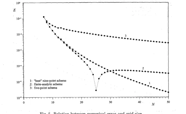
Fig. 5 Relation between numerical error and grid size.
grid elements with /:).x=/:).y=1!N, where N is an integer. The overall estimation of the numerical error is given by
Fig. 5 shows the relation betweenE andN. We note from this figure that, for the five-point scheme and the "best" nine-point scheme, the overall numerical error decreases continuously as the grid refined. The accuracy of the "best" nine-point scheme, however, is much higher than that of the five-point scheme at any fixed grid size and, more- over, it increases much more rapidly as the grid size is reduced. In other words, to get a solution of the same accuracy, the five-point scheme needs a much finer grid than the "best" nine-point scheme. We also note that the finite-analytic scheme is compa- rable to the "best" nine-point scheme only when a relatively rough grid is under consideration. The overall numerical error of the finite-analytic scheme does not show a monotonically reducing tendency as N increases. It decreases at a rate equivalent to or even more rapid than that of _the
"best" nine-point scheme as N increases up to a certain value (25 in the present case), but it decreases at a rate equivalent to that of the five-
1 j N N - ) 2
E= N+l ~o~o(¢m.n-¢m.n (37)
point· scheme as N becomes large. Since it is understood that the accuracy of the finite-analytic scheme depends on the representation of the varia- tion of the dependent variable along the boundary of grid element, we reckon that the formula for this representation adopted by Chwang and Chen (1987) is not necessarily good for a problem with fine grid.
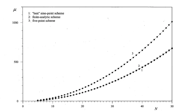
Fig. 6 shows the relation of the condition number in the above application of various schemes. Just as a confirmation to the analysis in the previous section, the five-point scheme .is shown to be dis- advantageous in terms of not only the accuracy but also the condition of difference' equation system.
Conclusions
We have studied the finite-difference schemes, including the classical five-point scheme, the finite- analytic scheme, and the "best" nine-point scheme, for numerical solution of the Laplace equation.
. The schemes, based on fairly different considera- tions were all formally represented bya. formula, that relates the nodal values of the dependent variable in a grid element. The coefficients of the schemes were expressed by different functions of the width-to-Iength ratio of the grid element. We demonstrated that there is an inherent contradic- tion in the finite-difference methods for the La-
1000 -
500 -
o o
1: "best" nine-point scheme 2: finite-analytic scheme 3 . five-point scheme
I I I I
10 20 30 40 50
N
Fig. 6 Relation between condition number of the difference equation system and grid size.
place equation. The grid size in an application must, on the one hand, be fine enough to ensure the numerical accuracy, but, on the other hand, be necessarily large to avoid an ill-conditioned differ- ence equation system. Higher-order schemes are shown to be advantageous in terms of both the accuracy and the condition of the difference equa- tion system.
References
1) Bickley, W. G. (1948). "Finite difference formu- lae for the square lattice", Quart.]. Mech. Appl.
Math., Vol. 1, 35-42.
2) Chen,c.]., Naseri-Neshat, H. andLi, P. (1980).
"The finite analytic method, Applications of analytic solution technique to numerical solu- tions of ordinary and partial differential equa- tions." Report ECjC-]-80, Dept. of Mech.
Engrg., Univ. of Iowa, Iowa City, lA, U. S. A.
3) Chwang, A.T. and Chen, H.C.(1987). "Optimal finite difference method for potential flows." ].
Engrg. Mech., ASCE, 113 (11), 1759-1773.
4) Fox,L. (1962). Numerical Solution of Ordinary and Partial Differential Equation; Pergamon Press, New York, NY, U. S. A.
5) Greenspan, D. (1957). "On the best9-point dif- fernece equation analogue of Laplace equa-
tion", ]. Franklin Inst., Vol. 264, 425-430.
6) Kantorovich, L. V. and Krylov, V. 1. (1958).
Approximate Methods of Higher Analysis, P.
Noordhoff Ltd., The Netherlands.
7) Lapidus, L. and Pinder, G. F. (1982). Numerical Solution of Partial Differential Equations in Science and Engineering, John Wieley& Sons, New York, NY, U. S. A.
8) Manohar, R. and Stepheson,J.W. (1982). "Opti- mal finite analytic methods", ]. Heat Trans., Vol. 104, 432-437.
9) Young, D. M. and Gregory, R. T. (1988). A Survey of Numerical Mathematics, Dover Publi- cation, New York, NY, U. S. A.