R&D-based Growth, Poverty Traps, and Multiple Steady States in an Endogenous
Growth Model with R&D Externality
∗Shiro Kuwahara † University of Hyogo
January 5, 2016
Abstract
Different economies seem to exhibit multiplicity with regard to economic paths. Upon facing severe economic shocks, some advanced economies experience a no-growth phase despite having had positive and occasionally high growth rates immediately before the shocks.
In contrast, many underdeveloped nations are stuck in a no-growth trap and their growth power is fragile, namely they sometimes en- counter big economic shocks after starting to develop. With the aim of integrative investigation of the mechanisms of these phenomena, this study develops a concise dynamic model involving monopolis- tic variety-expansion research and development (R&D) with the R&D spillover and capital R&D inputs. The model provides multiple steady states that contain high-, low-, and no-growth phases, each of which is selected by the expectations. Furthermore, high growth is impossible during early stages of development, and while low growth is globally possible, the dynamic property might show indeterminacy, and thus, the expectation formation contains some difficulties.
∗This work was conducted with financial support from JSPS KAKENHI Grant Number 15K03360, JSPS KAKENHI Grant Number 26380348, and the grant from Kobe Academic Park Association for the Promotion of Inter-University Research and Exchange.
†E-mail: [email protected] Phone/Fax: +81-78-794-5409
Keywords: multiple steady states; R&D-based growth; poverty traps; in- determinacy
1 Introduction
The classical study of Solow’s growth accounting (Solow 1957) showed that the source of long-run growth is TFP (total factor productivity) growth, where economies–especially, advanced countries–grow through technological progress driven by R&D activities. Although Solow’s result implies that economic growth can be promoted by technological progress, some empirical works such as Easterly (1994) and Quah (1996, 1997) have shown that the world economies are polarized into the rich and the poor, that is, many developing counties fall to grow and are stuck in a no-growth phase.
Furthermore, even the modern advanced countries confront several large shocks (e.g., the Japanese bubble collapse 1991, the dot-com bubble burst 2001, the 2008 financial crisis, and the European Debt Crisis 2010), and are often stuck in stagnation. In particular, the stagnation of Japan after the bubble collapse caused a long-run stagnation called ”the Lost Decade” or the
”Lost Two Decades”. Recently, some pessimistic views for economic growth such as Summers’ (2014) ”secular stagnation” have been proposed. As for the developing countries, while growth in some economies (e.g., the Four Asian Dragons and BRICS) has started, their fragility occasionally draws economic shocks, such as the 1997 Asian Financial Crisis. Thus, in the polarized global economy, not only newly developing economies but also advanced growing economies transit between positive and no-growth phases, which implies that the multiplicity of economic paths exists, and then, the change of expecta- tions caused by some economic shocks makes the economy jump between these. Thus, we aim to develop a model with the following properties: (i) a no-growth steady state without R&D, (ii) long-run steady states with R&D, and (iii) both steady states being possible and interchangeable.
As for the models that treat long-run no-growth and positive-growth steady states and a regime switch between them, we can refer to some the- oretical works describing the regime change from capital-based growth with decreasing returns to long-run positive growth1 (Zilibotti 1995; Matsuyama
1This phenomenon is empirically supported by Abramovitz and David (1973) and Hayami and Ogasawara (1999). By using US and Japanese data, respectively, they demon-
1999, 2001; Funke and Strulik 2000; Galor and Moav 2004; Irmen 2005;
Kuwahara 2007, 2013). The present study directly shares its structure with those of Matsuyama (1999, 2001) and Kuwahara (2007, 2013), who focus on the regime switch between capital-based and R&D-based growth.
Matsuyama (1999, 2001) contain two regimes, capital-accumulation-based growth and R&D-based growth, but their main concern is the business cy- cles between these two regimes. Next, Kuwahara (2013) yields a long-run, positive, or no-growth saddle-stable steady state, and therefore, the proper- ties (i) and (ii) stated above are obtained but condition (iii) is not. How- ever, Kuwahara (2007) obtains the result that a unique equilibrium without R&D exists under low capital stock, and after sufficient capital stock is accu- mulated, multiple equilibria (i.e., equilibrium with no, moderate, and large R&D input) emerge. Further, after adequate accumulation of capital, while an equilibrium again becomes unique, it is accompanied by R&D activities.
In other words, in Kuwahara (2007), multiplicity is a characteristic of the middle stage of economic development, and hence, analysis of condition (iii) is also insufficient.
To generate the global multiplicity, we introduce a slight modification on Kuwahara (2013) by considering that the R&D has a strong spillover on the small aggregate R&D input2. Thus, the steady states obtained in this study have no, low, and high R&D input. The obtained results are as follows.
Firstly, from the conditions for R&D, we show that globally, no R&D can be at equilibrium; therefore, even if a county is advanced, it has the possibility of falling in no-growth traps. Secondly, we have two types of equilibrium of positive R&D, namely middle and high R&D. For the middle R&D equilib- rium, the dynamical property of this regime might be indeterminacy, and it is possible to be selected globally, namely for all capital stock. For the high R&D equilibrium, this regime is saddle stable, but it is possible to be selected by the economy with sufficient knowledge-adjusted capital stock.
Thus, the equilibrium with middle R&D is the unique equilibrium for a de- veloping country, which does not have sufficient knowledge-adjusted capital stock, to grow through R&D. Consequently, the economic path with R&D for developing countries may fluctuate heavily.
strated that an economy mainly grows by capital accumulation at an early stage of the development and then shifts to growth by R&D activities.
2We can refer to Chu and Chen (2010) as a model introducing the spillover of R&D and deriving multiple steady states regarding R&D input.
The rest of the paper is organized as follows. Section 2 establishes the model of a decentralized economy. The existence of the two types of steady states and their determinants is explained in Section 3. The dynamic prop- erty of the model is analyzed in Section 4. Finally, Section 5 concludes the paper.
2 The Model
The present study adopts a Romer-type (Romer 1990) production structure.
It considers three sectors: final good, intermediate goods, and R&D. Fol- lowing Zilibotti (1995), we consider a composite durable good consisting of the private component of any reproducible private factor of production such as human and physical capital (simply called capital) with aggregate value K, and assume that it is used for either intermediate good production or R&D input3. Following Romer (1990), intermediate goods are patented, and therefore, supplied monopolistically.The number of the developed interme- diate goods is denoted as A, and inelastically supplied labor L, which is, therefore, regarded as the economy’s population scale, is assumed to grow at ecogenously given constant rate n. Each intermediate good is indexed by i, and ˜X(i) denotes the supply of the ith intermediate good. The number of the intermediate-goods cluster—the variety of intermediate goods—denoted by A, therefore it is i ∈ [0, A]. and since all types of intermediate goods is used in poduction of final goods, A represents the technological level in the economy, and can be regarded as the level of knowledge accumulation, or knowledge capital. Final good is consumed as a consumer good or invested as capital. Capital is used as an intermediate good for supplying the final good sector (KY) and for investment to create new intermediate goods, that is, R&D (KA). Accordingly, the market-clearing condition for capital imposes K =KY +KA, where K is the amount of capital in the economy. Time is continuous, and the final good is taken as the num´eraire.
In this papaer, we use capital laterZ as an aggregate variable, and forZ, define as follows: z ≡ Z/L, ˜Z ≡ Z/A, and ˜z ≡ Z/(AL), which respectively imply per capita, knowledge-adjusted, and knowledge-adjusted per capita value of Z.
3See Kuwahara (2013) for an explicit treatment of human capital. The main working of the capital derived in it is essentially similar to that of our one-type capital model.
2.1 Production
The production function of the final good is Y =L1−α
Z A
0
x(i)αdi, 0< α <1, (1) where Y denote final good production. Intermediate goods are produced us- ing physical capital and are used for producing the final good. One unit of intermediate goods is assumed to be produced by η units of capital.
Therefore, the capital allocated to the production of final good KY is quan- tified as KY ≡ RA
0 ηX(i)di. An assumption of symmetric equilibrium re-˜ garding intermediate goods, that is, ˜X = ˜X(i), converts the quantification of K into KY = ηAX, or equivalently, ˜˜ X = (1/η)(KY/A). Substituting X(i) = ˜˜ X = (1/η)(KY/A) into Eq. (1), we have reduced final good pro- duction function as Y =η−αA1−αKYαL1−α4. Using Y derived above and the assumption that final goodY is consumed or invested, we yield the following resource constraint for the final good:
K˙ =η−αKYαA1−αL1−α−C(=Y −C), (2) where ˙KandCdenote an increment in aggregate capitalKand consumption, respectively.
The final good sector is competitive, and Eq. (1) yields the first-order conditions (FOCs) for final good production. These are given as ∂x(i)∂Y =p(i), where p(i) denotes the price of intermediate good i.
In our model, intermediate goods are protected by patents, and a firm holding a patent for the production of the ith intermediate good can be designated as a supplier of the ith intermediate good. Thus, the ith inter- mediate good is supplied monopolistically by the ith firm. Since we assume that one unit of an intermediate good is produced using η units of capi- tal, the profit of the firm producing the ith intermediate good is given as Π(i)˜ ≡ p(i) ˜X(i)−rηX(i), where˜ r is the rental price of capital. Under the assumption of symmetric equilibrium, the firm producing an intermediate good maximizes this profit subject to ∂x(i)∂Y =p(i). This optimization condi- tion yields the following: ˜X(i) = ˜X =
³α2 rη
´1−α1
and p(i) =p=¡η
α
¢r, where
4It should be noted that the parameterαthat determines capital/labor share is larger than the usual case whereK is assumed to be composed by only physical capital.
X˜ =X/A means per patent value. Applying the notation ˜z to Y, r, and ˜Π, and using Eq. (1),KY =ηAX, and the FOCs, we obtain knowledge-adjusted˜ output ˜y, interest rate r, and the knowledge-adjusted per capita profit from the production of intermediate goods ˜π, respectively, from the following:
˜
v =η−α˜kαY, r=α2η−α˜kαY−1, and π˜= ˜π(i) = (1−α)αy,˜ (3) where, in equilibrium, the profit of each firm producing an intermediate good is equalized; therefore, we can write π=π(i).
2.2 Innovation
R&D firms create new intermediate goods, and each innovation obtains the perpetual patent that yields a perpetual sequence of monopoly profits π, which comprise the revenue of R&D. Thus, the present value of this stream represents the value of R&D5: ˜Vt≡R∞
t Π(τ)e˜ −Rtτr(s)dsdτ.Free entry of R&D is assumed. Therefore, if revenue from R&D exceeds its costs, an infinite amount of capital would be allocated to it. Thus, revenue from R&D cannot exceed the cost in equilibrium, and if this is achieved, investment in R&D is unprofitable, and no resources are allocated to R&D. In this case, an equilibrium without R&D (KA = 0) occurs. Thus, if the economy is in equilibrium with positive R&D investment, the revenues generated by R&D must be equated to its cost.
Since we assume that capital is invested to undertake R&D, firms that engage in R&D must pay a rental cost r for their R&D activities in the pro- cess of innovation. Furthermore, innovation is assumed to be the discovery of new intermediate goods that are added to the existing set of intermediate goods; therefore, the expansion of variety can be shown by the time deriva- tion of knowledge capital, ˙A. Thus, the aggregate value in the economy is the summation of all of these firms, ˜V A; the aggregate innovated value by R&D and its input cost are given as vA˙ and rKA, respectively, and the free entry on R&D equates these two, and thus, the relationships between market equilibrium and capital allocation are summarized as
Solow Regime: KA= 0 Romer Regime: KA>0
)
⇐⇒r(t)KA(t) (
>
= )
V˜(t) ˙A(t). (4)
5We define the aggregate value of firms and profits as follows: V ≡ RA
0 V˜(i)di, and Π≡RA
0 Π(i)di, respectively.˜
Whether an economy conducts R&D depends on condition (4). WhenKA>
0, R&D occurs, causing the economy to grow through endogenous techno- logical change. Following Matsuyama (1999), we term this regime as the Romer regime. Condition (4) states that equality rKA = ˜VA, or˙ rk˜A=gAv, wheregZ ≡Z/Z, holds in the Romer regime. When ˜˙ kA= 0, no R&D occurs, and the economy grows only by capital accumulation. Following Matsuyama (1999), we term this as the Solow regime.
Following each regime, differentiating ˜V with respect to time provides the following asset equations:
Solow Regime: K˜A= 0 Romer Regime: K˜A>0
)
⇐⇒r(t) ˜V(t) (
>
= )
Π(t) +˜ V˙˜(t). (5) If R&D is undertaken, technological knowledge is assumed to increase according to per capita capital investment in R&D. We assume that the R&D function is as follows:
A˙ = φ(t)
Γ(t)A(t)KA(t),
where φ is the R&D efficiency. and Γ captures the factor that eliminates scale effects in this model. If ˜φis assumed to be constant, the case is similar to that of the Romer-type technology: innovated R&D linearly depends on R&D input. To obtain the existence of steady states, we simply assume that Γ(t) = A(t)L(t), and the above equation is made as
gA(t) = φ(t)˜kA(t). (6)
Funke & Strulik (2000), which shares the R&D structure of endogenously accumulated (human) capital as R&D input, also adopt a technology that is essentially the same type.
One shortcoming for our concern in the analysis of the no-growth trap is the constant return of R&D, which assures efficiency of R&D6. Therefore, we assume that φ is an increasing function for a sufficiently small R&D input:
Assumption on R&D Property While the return is assumed to be con- stant and positive over the domain with sufficient R&D input, we introduce
6Therefore, the Jones technology (Jones 1995) also has the same shortcoming. It has infinite large marginal efficiency for the R&D input tending to 0.
slightly increasing returns from knowledge spillover of R&D activities. Thus, R&D efficiency φ is continuous for ∀˜kA ≥ 0 and decreasing to 0 as social R&D input tends to 0, and we specify φ as follows:
φ=
δ, δ >0 for ˜kA> κ φ(˜kA), φ0(·)>0 for ˜kA∈[0, κ]
0, for ˜kA= 0
where φis the function with a threshold valueκ, above which, it is constant at δ, and sinceφis assumed to be continuous, we assume thatlim˜kA→0φ(˜kA) = 0 and lim˜kA→κφ(˜kA) =δ.
The picture ofφ is depicted in Fig. 1. The parameterδ represents R&D efficiency and is constant on almost all domains but increasing in the small R&D input. Thus, marginal R&D efficiency is smaller on near 0 R&D input.
To complete the model, we examine the consumption decision of house- holds. It is assumed that a representative household has a normal CRRA (constant relative risk aversion) type utility. Then, the Euler equation is obtained as θgc(t) =r(t)−n−ρ, wherec, θ and ρ, respectively, denote per capita consumpotion, the CRRA parameter and subjective discount rate.
3 Steady States
We now analyze an economy in a steady state, wherein all variables, Y, C, K, KY, and A, grow at constant rates, and therefore ˜y, ˜c, ˜k, and ˜kY are constant. Our model contains two types of steady states: one with R&D (and therefore, positive growth) and the other without R&D (and therefore, no growth). We call these types of states the Romer steady states (RSS) and the Solow steady states (SSS), respectively. Eqs. (4) and (6) yield
˜
v(t) = r(t)
φ(t). (7)
Eqs. (2) and (3) imply that gssy = gkss = gcss = gAss +n, where index ss represents the value of the steady states. Substituting gssc = gAss and gA=φ(˜kA)˜kA into the Euler equation, we obtain one conditional equation:
rss =θφss˜kAss+ρ+n. (8)
In the steady state, gvss˜ = gπss˜ = 0 holds because ˜kss is constant, and therefore, gvss˜ = 0. Substituting these relationships, that is, substituting Eqs. (3), (7), and (8) into Eq. (5) yields the following condition for R&D:
Romer Steady States (RSS):
Solow Steady States (SSS):
)
⇐⇒
ρ+n+θφss(˜kssA)˜kssA =α2η−α˜kYss α−1+n (
=
>
)
φ(˜kssA)1−α α
k˜Yss. (9) First, we characterize the SSS. In the SSS, Eq. (9) holds with inequality and all capital is devoted to the production of the final good. Therefore, k˜A∗∗ = 0; that is, k∗∗ = ˜k∗∗Y and g∗∗A = 0, where ∗∗ denotes the steady state value in the SSS. Substituting this into the Euler equation yieldsr∗∗=ρ+n, which along with rin Eq. (3) yields the equilibrium capital stock in the SSS:
SSS: ˜k∗∗ = ˜kY∗∗=
·α2η−α ρ+n
¸1−1α .
Under the assumption of φ (See Fig. 1), the second and third terms of Eq.
(9) imply that the second term is always positive, and the third tends to 0.
Thus, we immediately obtain the following lemma:
Lemma 1-1 The SSS is always possible.
It should be noted that this property stems from lim˜kA→0φ(˜kA) = 0.
3.1 Property of the RSS
Next, we investigate the properties of steady states with positive R&D input.
As is obtained below, we consider two equilibria, with large and small R&D inputs, respectively denoted by RSS(+) and RSS(–). The first and third terms, and first and second terms of Eq. (9) respectively yield the following two equations:
k˜= µ
1 + αθ 1−α
¶
˜kA+ α(ρ+n)
1−α φ(˜kA)−1¡
≡Φ1(˜kA)¢ , k˜= ˜kA+
· α2η−α ρ+n+φ(˜kA)˜kA
¸1−1α¡
≡Φ2(˜kA)¢ .
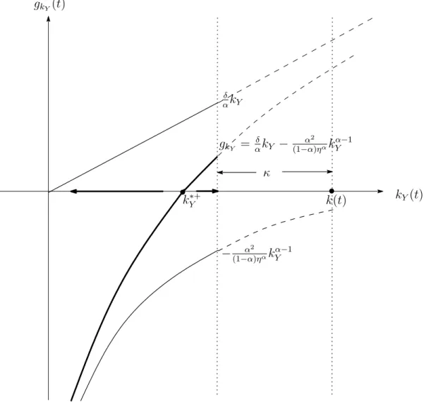
The curves of these two equations are depicted in Fig. 2. The intersection points of these two equations, Φ1 and Φ2, enable the two equilibria for ˜kA to be greater than 0. For κ <k˜A, φ =δ makes Φ1 a linear function defined as Φ¯1 ≡¡
1 + 1αθ−α¢˜kA+(1αρ+n−α)δ, Φ2 asymptotically moves close to ¯Φ2(˜kA)≡k˜A+ hα2η−α
ρ+n
i1−1α
from the above of ¯Φ2, and ˜Φ1 has steeper angle than ¯Φ2, hence, Φ¯2(κ) > Φ¯1(κ) is the necessary and sufficient condition for the equilibrium of R&D input larger than of κ (which we call RSS(+)) to uniquely exist, and the equilibrum value of R&D input is denoted as ˜kA∗+. The condition Φ¯2(κ) > Φ¯1(κ) is rewritten as δ > Ω under κ < κ, where¯ δ > Ω is derived from ( ¯Φ2(0) ≡)φ2 > φ1(≡Φ¯1(0)), and we define
Ω≡ α−1+α1−αη1−ααρ(ρ+n)1−1α
1−α , and κ¯≡arg (
κ
¯¯¯¯
¯
·α(ρ+θδκ) (1−α)δ
¸1−α
= α2η−α ρ+n+δκ
) . It should be noted that ¯κ > 0 is satisfied. It can be clearly observed that
k˜Y∗+ > κalways and uniquely exists as long as a feasible condition ˜kY ∈(0,˜k]
is satisfied. From ˜k = Φ2(˜kA) and ˜k = ˜kY + ˜kA, we obtain the equilibrium capital allocation to the production of the final good in RSS(+): ˜k∗Y+ =φ2.
When δ >Ω holds, we further have the possibility of the steady state on k˜A ∈(0, κ), which has smaller R&D input than RSS(+), so we call it RSS(–).
Since Φ1(κ)<Φ2(κ), lim˜kA→0Φ1(˜kA)>lim˜kA→0Φ2(˜kA), and continuousφ(·), there is at least one intersection of Φ1 and Φ2. Furthermore, if the intersec- tion locates in the domain ˜k > ˜kA, the steady state is feasible. Hereafter, we assume that there is one steady state of RSS(–), which is obtained, for example, by assuming thatφ is an exponential function with constant power (exponential coefficient). Thus, we obtain the following lemma.
Lemma 1-2 For the existence of RSS, the following parameter condition should hold:
δ >Ω(ρ, n, α, η), κ <κ(δ, ρ, n, θ, α, η),¯ ⇔ RSS(+) is feasible.
namely, sufficiently small κ and sufficiently large R&D parameter δ yields RSS(+). In this case, at least one equilibrium with less R&D input also ex- ists. We name this equilibrium RSS(–), and for smaller κ, the corresponding smaller k˜∗A exist.
Proof) The last part of the above lemma is proved as follows: Feasible con- dition is Φ1(κ) < Φ2(κ) and limk˜A→0Φ1(˜kA) = ∞ > ˜k∗∗ = lim˜kA→0Φ2(˜kA).
(Q.E.D)
We respectively call the Romer(+) regime and Romer(–) regime the growth phase converging RSS(+) and RSS(–).
3.2 Determination of the Steady State
We call the steady-state type of the economy with δ > Ω as the multiple steady state (MSS), because the economy withδ >Ω satisfies the conditions for the RSS(+/–) and the SSS always exists. As for an economy with δ <Ω, it has only the SSS. Accordingly, the emergence of steady state(s) is uniquely determined by the economy’s parameter set {δ, κ, ρ+n, θ, α, η}. Thus, the determination of the steady state is summarized in the following proposition.
Proposition 1: Under a sufficiently small κ, an economy has either mul- tiple steady states or only poverty trap, depending on the following parameter condition:
δ (
>
<
)
Ω(η, ρ, n, α)⇔ (
MSS (RSS+SSS) SSS.
This proposition implies that deep parameters determine the growth rate in the long-run: small ρ+n and large δ lead to the RSS. Intuitively, these results imply that a country with higher R&D efficiency and more patience has the possibility to realize the RSS, that is, long-run R&D-based growth.
However, this proposition also implies that any country has possibility stuck in the SSS, that is, although a country has a sufficiently high R&D efficiency parameter, it always has the possibility to be caught in the poverty traps.
Because the purpose of this study is the multiplicity of steady states in the developed countries, namely countries that can grow with innovation (at least, potentially), we later assume that RSS is possible, that is, δ > Ω (or equivalently, Ω/δ <1) holds. Further, for simplicity, we assume that RSS(–) uniquely exists.
In this situation, we have the following lemma about the steady-state knowledge-adjusted capital accumulation:
Lemma 1-3 The knowledge-adjusted capital allocated to the production sec- tor in SSS, RSS(–), and RSS(+) have the following order:
k˜Y∗∗(= ˜k∗∗)>˜k∗Y− >k˜∗Y+.
Proof. From steady-state values, we have ˜k∗∗= ˜kY∗∗ =
hα2η−α ρ+n
i1−α1
, ˜kY∗− = h α3
(1−α)ηαφ(˜k∗−A )
i2−1α
, and ˜kY∗+ =
h α3 (1−α)ηαδ
i2−1α
. Then, from the proof of the Lemma 1-2, we already obtained ˜kY∗∗(= ˜k∗∗)>k˜∗Y−. (Q.E.D.)
4 Transition Dynamics and Steady States
In this section, we analyze transition dynamics. On the transition path, we have two regimes, characterized as ˜kA>0 and ˜kA = 0. We call them as the Romer regime and the Solow regime, respectively.
4.1 Local Transition Dynamics
An economic system comprises Eqs. (2), (3), (4), the Euler equation and the equation in condition (9). We reconstruct this into a system comprising k, c, and ˜kY. SubstitutingY andr given in Eq. (3) into Eq. (2), we obtain the dynamics of k:
k(t) =˙˜ η−αk˜Y(t)α−˜c(t)−n
φ(t)¡k(t)˜ −˜kY(t)¢ +n
ok(t).˜ (10)
Further, substitutingg˜c+gA=gcandr=α2η−αk˜Yα−1into the Euler equation, we obtain the dynamics of cas follows:
˙˜
c(t) = 1 θ
©α2η−α˜kY(t)α−1−ρ+n−θφ(t)(˜k(t)−k˜Y(t))ª
˜
c(t). (11) These two dynamics are common to the two regimes. In the case of ˜kY, each regime follows different dynamics as described below.
4.1.1 Dynamics of the Economy in the Solow Regime
First, we investigate the Solow regime characterized by condition ˜kA = 0, which directly leads to k(t) = kY(t) and A(t) = ¯A. Thus, the Solow regime also exists on a two-dimensional plane, which we call the Solow- regime manifold. Under this condition, the system comprising Eqs. (10) and (11) is changed such that it comprises ˙k(t) = η−αA¯1−αk(t)α−c(t) and
˙
c(t) = 1θ©
α2η−αA¯1−αk(t)α−1 −ρ−nª
c(t). Thus, the dynamic system in this
case is similar to that of the normal Solow model. One difference is the interest rate, because the Romer-type R&D-based growth model contains distortional intermediate goods pricing. However, the dynamic properties are essentially the same as the normal Solow model.
Lemma 2-1 The Solow regime is globally possible, and the SSS is saddle- path stable.
Proof. See the Appendix.
4.1.2 Dynamics of the Economy in the Romer Regime
Next, we examine the Romer regime, which is the steady state with KA>0.
From Eq. (7) and the equation in (9), we obtain gr−gφ =r− δπr . Then, r and ˜π derived in Eq. (3) yield gr = (α−1)g˜kY and δπ/r˜ = δ(1−α)˜kY/α.
Substituting these two equations intogr−gφ=r−δ˜rπ, we obtain the dynamics of ˜kY as
k˙Y(t) = φ(t) α
˜kY(t)2− gφ(˜k(t)−˜kY(t)) 1−α
k˜Y(t)− α2η−α 1−α
k˜Y(t)α. (12) We have two regimes of the value of φ; one is named by the Romer (+) regime, where φ(t) = δ (constant), and the other by the Romer(–) regime, where φ(t) is variable.
Under the Romer(+) regime, imposing φ(t) = δ and ˙φ(t) = 0 on (12) yields k˙˜Y(t) = αδ˜kY(t)2 − α12−η−αα ˜kY(t)α. Because the dynamics of ˜kY guided by this reduced equation is the function that contains only ˜kA, the dynamic properties of ˜kY are directly obtained, and the dynamics of ˜kY are found to be unstable around ˜kY∗, as is given in Fig. 3. In the Romer(+) regime, knowledge-adjusted capital allocated to final goods ˜kY(t) is necessary to be constant at ˜kY(t) = ˜kY∗+ and therefore, knowledge-adjusted capital stock is necessary to be sufficiently large, that is, ˜k(t) > k˜∗Y+. We call the plane k˜Y(t) = ˜k∗Y, on which the economy in Romer(+) regime transits, as the Romer(+)-regime manifold. Thus, the Romer regime with RSS(+) is de- picted on a two-dimensional plane {˜k(t),c(t)˜ }, and considering this property and (10) and (11), RSS(+) is conformed as having saddle-path stability (See Appendix).
On RSS(–),φis variable. We define σ≡ φφ(˜0(˜kkA)˜kA
A(t)) and assume thatσ is, at
least, constant around the RSS(–). Under this setup, we have the following:
k˙˜Y(t) = Ψ(t)
"
− α2
1−αη−α˜kY(t)α+φ(˜kA(t)) α
k˜Y(t)2
− σk(t)˙ (1−α)˜kA(t)
˜kY(t)
#
. (13)
where Ψ≡ (1−(1α)(˜−α)(˜k−k˜kY−)˜k−Yσ)˜kY(>1). Because ˜kA =k−˜kA, the system is depicted by three variables {k,˜ ˜c,k˜Y}. Thus, the linearized system of the Romer(–) regime around the steady state are given by Eqs. (10), (11), and (13), and the Appendix shows that the system has a positive determinant. Thus, if the system has a negative trace, it has an indeterminacy property, which is obtained, for example, by a sufficiently large externalityσ: see the Appendix for detail analysis of the dynamic properties of the Romer(–) regime. Differ- ent from the RSS(+), the Romer (–) regime does not contain the threshold value and is possible at any initial value of knowledge-adjusted capital stock.
Lemma 2-2 The Romer(+) regime is possible for k(t)˜ > k˜Y∗+ and the Romer(–) regime is possible for any capital stock level. The RSS(+) has saddle-path stability, and the RSS(–) shows indeterminacy for sufficiently large externality parameter σ.
4.2 Global Transition Dynamics and Steady States
Combining the local transition dynamics and the steady state condition dis- cussed in the previous section, we here derive the global dynamics in the present study.
From the above discussions, the basic development process is described as follows. If the economy has RSS(+) and expects this to be the steady state of the economy but has smaller initial knowledge-adjusted capital than the threshold value ˜k∗Y+, then the economy cannot ride on the Romer(+) regime at the early stage. This is because from Lemma 2-2, the transition path con- verging to the RSS(+) needs larger knowledge capital than ˜k∗Y+. Thus, until the economy accumulates capital ˜k= ˜kY∗, the economy grows by only capital accumulation, and after reaching the threshold value ˜kY∗, it grows by techno- logical progress through R&D. This is the process of economic development