Statistical considerations for design and analysis of comparative clinical trials

(1)

Statistical considerations for design and analysis of comparative clinical trials

Keika Okawa

September 28, 2018

(2)

- 1 -

Chapter 1 Background and introduction

In clinical research, biostatisticians are deeply involved from the design stage of the trial, and they propose and advise on the study endpoint, statistical analysis plan, the sample size, and so on. Among various types of design for clinical research, particularly in phase III comparative clinical trials to confirm the efficacy and safety of new pharmaceutical products, ingenuity for clinical trial design is crucial to place the products with social benefits on the market as soon as possible. Furthermore, statistical analysis methods and study endpoints adopted in the trial should be reasonable and valid in the light of the characteristics of the targeted therapy.

Recently, various types of study designs have been proposed to overcome the complicated situations encountered in clinical trials. This thesis focuses on two subjects related to statistical considerations on the study design and analysis method in comparative clinical trials.

In Chapter 2, I propose a new monitoring tool for interim analysis. Interim analyses are often planned in randomized clinical trials for possible early trial termination to claim superiority or futility of a new therapy. The proposed blinded data monitoring tool enables investigators to predict whether they observe such an unblinded interim analysis results that support early termination of the trial. Investigators may skip some of the planned interim

(4)

- 3 -

analyses if early termination is unlikely. Here, this thesis specifically focused on blinded, randomized-controlled studies to compare binary endpoints of a new treatment with a control. Extensive simulation studies are conducted to assess the impact of the implementation of our tool on the size, power, expected number of interim analyses, and bias in the treatment effect.

Then in Chapter 3, I discuss issues of conventional cancer trial design and analysis and present alternatives to the hazard ratio (HR) using a recent immunotherapy study, i.e., the restricted mean survival time (RMST). In a comparative cancer clinical study with progression-free survival (PFS) or overall survival (OS) as the endpoint, the HR is routinely utilized to design the study and then to estimate the treatment effect at the end of the study.

The clinical interpretation of HR may not be straightforward, especially when the underlying model assumption is not valid. A robust procedure for study design and analysis that enables clinically meaningful interpretation of trial results is warranted. This thesis first discuss issues of using HR and present RMST as a summary measure of patients’ survival profile over time. This thesis then shows how to use the difference/ratio in RMST between two groups as an alternative for designing and analyzing a cancer clinical study via an immunotherapy study as an illustrative example.

Finally, concluding remarks are given in Chapter 4.

(5)

4

Chapter 2 Decision on performing interim analysis for comparative clinical trials

2.1 Introduction

In randomized-controlled trials, interim analyses are often planned to review the efficacy or safety of the therapeutic interventions. Early termination of the trial may occur due to evidence of superiority or futility of the new therapy based on the interim analysis. To conduct interim analyses, we need to access the data prior to the completion of the trial. Particularly for blinded studies, interim analysis requires unblinding of the treatment allocation and conducting a formal between-group comparison^1,2. Although unblinded data provide complete information of the observed data, blinded data also contain information about the treatment difference between the groups. For instance, when the observed response rate in the pooled sample is very low at the time of the interim analysis, we know the response rates in both groups are very low. Therefore, there is little chance a significant difference between the groups would be observed and, consequently, a formal comparison is a wasteful expenditure of alpha. Even when response rates are not that small, if the control rate can be reasonably estimated based on previous studies, the blinded data yields a decent estimate of the treatment difference.

There are several data monitoring tools^3-5 that use blinded data originating in the Bayesian approach for safety monitoring in single arm studies proposed

(6)

5

by Thall and Simon⁶. For example, Ball³ focused on the adverse event rate in the pooled sample and proposed a decision rule based on the posterior distribution of it using the Bayesian approach. On the other hand, our focus in this paper is a blinded data monitoring tool predicting the result of a formal unblinded interim analysis for superiority or futility of a new therapy. The proposed tool works with the hypothesis testing approach. Specifically, we assume that the alpha spending function approach⁷ is used as a stopping guideline for superiority in the formal interim analysis. For futility, we assume that the result of stochastic curtailment method is used as a guideline of early stopping⁸. We performed extensive numerical studies to assess the impact of the implementation of the data monitoring tool on the type I error rate, power, expected sample size, expected number of interim analyses to be performed and bias in the treatment effect for both superiority and futility.

We illustrated the practical application of our tool, using data from a clinical trial conducted by the ECOG-ACRIN Cancer Research Group. With our tool, investigators may skip some of the planned interim analyses when the result of an interim analysis at that time point is unlikely to support early termination of the trial for superiority or futility. Therefore, this tool could ultimately avoid unnecessary spending of study resources while maintaining scientific integrity of the trial.

(7)

6

2.2 Blinded data monitoring tool

In this paper, we specifically focus on randomized controlled trials comparing binary endpoints, namely response rates, between a new therapy and a control. In the trial, interim analyses are planned for early termination for superiority or futility or both.

2.2.1 Typical procedure of interim analysis

Usually, the interim analysis is implemented at the time when the pre- planned information fraction is reached. For a binary outcome, the total information will be defined as the planned total sample size. Assume that, during the accumulating the preset sample size M, there are N (≤M) participants and T (≤N) responders in the two arms at the time of the interim analysis. Let (𝑇₁, 𝑇₀) denote the numbers of responders in the arm of the new therapy and control respectively, and then 𝑇 = 𝑇₁+ 𝑇₀. When unblinding the data, we can observe (𝑇₁, 𝑇₀), and formal comparison would be implemented.

Depending on the resulting test statistic, or the corresponding p-value or conditional power, we decide whether to stop or continue the trial.

2.2.2 Blinded data monitoring tool

Before breaking the blinded treatment assignment code, we may monitor (𝑁, 𝑇) from the blinded data. Assume that each 𝑇₁ and 𝑇₀ follows a

binomial distribution with a parameter 𝑝₁ for the new therapy and 𝑝₀ for the control therapy, respectively. The probability mass function of 𝑇, 𝑃𝑟(𝑇 = 𝑡), can be expressed with a mixture of the aforementioned two binomials.

Given the allocation ratio during the study 𝑞: (1 − 𝑞) for the new therapy and control respectively, where 𝑞 ∈ (0,1), 𝑃𝑟(𝑇 = 𝑡) is expressed that

(8)

7

𝑃𝑟(𝑇 = 𝑡) = (𝑁

𝑡) {𝑞𝑝₁+ (1 − 𝑞)𝑝₀}^𝑡{𝑞(1 − 𝑝₁) + (1 − 𝑞)(1 − 𝑝₀)}^𝑁−𝑡. With the blinded treatment allocation, if we have enough certainty about 𝑝₀ and if the allocation ratio is close to 𝑞, we would be able to predict the

response rate of the new therapy 𝑝₁. Specifically, if 𝑝₀ is a known value, the maximum likelihood estimator of 𝑝₁ is obtained by

𝑝₁

̂ = 𝑇 − 𝑁(1 − 𝑞)𝑝₀

𝑁𝑞 .

Then the standardized test statistics for testing the null hypothesis 𝐻₀: 𝑝₁ = 𝑝₀ is given by 𝑍_𝑏 = (𝑝̂ − 𝑝₁ ₀)/√Var̂ (𝑝̂), where ₁ Var̂ (𝑝̂) = 𝑁𝑟̂(1 − 𝑟̂)/(𝑁𝑞)₁ ² and 𝑟̂ = 𝑞𝑝̂ + (1 − 𝑞)𝑝₁ ₀. Utilizing the observed 𝑍_𝑏 at the interim analysis point, we can predict whether or not the unblinded interim analysis result will meet the stopping criteria for superiority or futility. For superiority, one can then obtain the threshold values of the total number of responders 𝑇 with respect to each number of subjects 𝑁, with which the 𝑝-value of the test would meet the pre-specified stopping criteria corresponding to the information time at the interim analysis. For futility, one might use a conditional probability as criteria for stopping.

2.2.3 Illustrative example

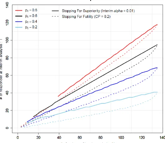
To illustrate the aforementioned decision criteria, we consider a specific numerical example of a randomized controlled trial comparing response rates between the new and the control therapy. The accrual goal is 135 patients and the mixture proportion of allocation is 𝑞: (1 − 𝑞) =²₃∶ ¹₃ for the new therapy and the control, respectively.

(9)

8

First, we consider the case for interim analysis expecting early termination only for superiority and consuming type I error rate 𝛼 = 0.01 at the interim analysis. Under this scenario, the solid curves in Figure 1 show the

thresholds of 𝑁 and 𝑇 with various values of 𝑝₀. For example, the blue solid curve corresponds the case that 𝑝₀ = 0.4. Using the observed (𝑁, 𝑇) with blindness maintained, these curves can be a reference to predict how likely the interim analysis result would meet the stopping criteria, if conducted. Specifically, in this example, when the observed (𝑁, 𝑇) is above the blue curve, we can expect that the result of the interim analysis will support early stopping for superiority for the new therapy. Therefore, if we think that 𝑝₀ is very likely to be 0.4, we would conclude that an interim analysis should not be missed at this point.

Next, we consider the case of early termination for futility based on the conditional power less than 0.2. The dashed lines in Figure 1 show the corresponding N-T curves for futility with various 𝑝₀′𝑠. Again, consider the case that 𝑝₀ = 0.4. The observed (𝑁, 𝑇) below the blue dashed curve

indicates the conditional power will likely be below 0.2. Thus, if we are confident with a 𝑝₀ = 0.4, we would determine the interim analysis should not be missed for potential futility stop. On the other hand, if the observed (𝑁, 𝑇) is above the blue dashed curve, it may be an option to skip the scheduled interim analysis, if there are no other concerns on the study.

This tool can also be used for the cases that both superiority and futility stoppings are of interest. In those cases, we will use both solid and dashed curves in Figure 1. When the observed (𝑁, 𝑇) is in between solid and

(10)

9

dashed lines, the interim analysis result will likely not meet stopping

criteria for either superiority or futility. We may skip performing the interim analysis and continue the trial, unless there are other concerns in the study.

In this manner, the proposed blinded monitoring process is helpful for

identifying whether it is a good time to conduct interim analysis, preserving the integrity of the study. Appendix 1 provides the computer programs to generate N-T plots with a documented example.

Figure 1. N-T plot with 𝐩𝟎= 0.8, 0.6, 0.4 and 0.2 for early stopping for superiority and futility.

(11)

10

2.3 Simulation studies

We performed extensive numerical studies to assess the impact of the

implementation of the proposed blinded data monitoring tool with respect to a randomized controlled design using 2:1 allocation (new therapy : control) and comparison of a binary outcome. We assume that the investigators plan to do one interim analysis when the outcome of 60 patients are available among the planned 135 patients. The overall type I error rate is set to 0.05.

We consider that 0.01 of the alpha would be spent at the interim analysis, and then the critical p-value for the second analysis is derived to be 0.0446 by the Hybittle-Peto method [9,10]. The true response rates of the new therapy 𝑝₁ were set to 0.40, 0.50, 0.60, 0.65, 0.70 and 0.80, and the true response rate of the control group 𝑝₀ was set to 0.40. The binary outcomes are generated from the binomial distribution with the success probability 𝑝₁ for the new therapy and 𝑝₀ for the control arm, respectively. Iterating 10000 times, we assessed the overall type I error rate, power, expected sample size, the probability of conducting the interim analysis, the

probability of stopping the trial at the interim analysis, and the bias of the treatment effect.

In these simulations, three patterns of early termination criteria were evaluated--- 1) only for superiority, 2) only for futility, and 3) both for superiority and futility. Within each pattern, four scenarios as outlined below were considered.

 First scenario (Without using our tool)

As a conventional procedure of randomized controlled trials, an interim

(12)

11

analysis is conducted at a pre-specified information time. If the result of the interim analysis is significant, we stop the study for superiority of the new therapy. Otherwise, the trial will be continued until full accrual, and the second analysis conducted with the planned sample size.

 Second scenario (Using our tool with a correct 𝑝₀)

At the pre-specified time point in the aforementioned scenario, the decision of whether or not to conduct an interim analysis is made by the proposed blinded data monitoring tool with a correctly specified parameter for the control arm. When our tool suggests an interim analysis should be

conducted, the interim data will be unblinded and the interim analysis will be performed as in the first scenario. On the other hand, when our tool suggests skipping the interim analysis, the data will be analyzed only at the end of the trial. In the latter case, since we haven’t spent alpha for the interim analysis, the nominal level of the type I error rate is used at the final analysis.

 Other scenarios (Using our tool with mis-specified 𝑝₀)

We take the same procedure as described in the second scenario, but consider the case when 𝑝₀ is misspecified when creating N-T plot. Specifically, we consider a case where we underestimate 𝑝₀ (i.e., 𝑝₀ = 0.30 in the third scenario ‘lower’ 𝑝₀ ) and a case where we overestimate 𝑝₀ (i.e, 𝑝₀ = 0.50 in the fourth scenario).

2.3.1 For case of early termination for superiority

Table 1 presents the simulation results in the case of early termination for

(13)

12

superiority at the one interim analysis which is done with 60 patients. In this table, we report power or size (overall type I error rate), the expected sample size during the study (E[M]), the probability to conduct an interim analysis (IA), the probability to terminate the trial at the interim analysis for superiority of the new therapy (Sig.IA), and the proportion of Sig.IA/IA, among 10000 sets of samples. Note that the expected sample size would also be an indicator of the expected study duration. When the expected sample size is close to 135, the study would be continued until the time of the final analysis. We also evaluated the bias of the treatment effect via E[𝑝̂ − 𝑝₁ ̂] −₀ (𝑝₁− 𝑝₀). Scenario 1-1 shows the results of the case using the conventional strategy and the other three scenarios show the results using the proposed blinded data monitoring tool under various conditions of 𝑝₀.

(14)

13

(15)

14

2.3.2 For case of early termination for futility

In this setting, we consider early stopping for futility, instead of superiority.

Specifically, at the planned interim analysis time point, we calculate the conditional probability. If it is below 0.2, we stop the trial. The incorporation of a futility stopping rule affects the overall type I error, but we do not adjust for it in this numerical study. Therefore, the critical p-value at the final analysis is 0.05. In Table 2, we report the probability to terminate the trial at the interim analysis for futility of the new therapy (Fut.IA), and the proportion of Fut.IA/IA, in addition to power or size (overall type I error rate), the expected sample size during the study E[M], IA and the bias of the treatment effect under each four data monitoring scenario.

(16)

15

(17)

16

2.3.3 For case of early termination for superiority and futility

We now consider the case with both superiority and futility stopping rules.

Specifically, at the interim analysis, we will stop the trial for superiority if the observed p-value is less than 0.01, or for futility if the conditional probability is less than 0.2. Table 3 gives the results of the four data monitoring scenarios including the parameters power and size, E[M], IA, Sig.IA, Fut.IA, the proportion of Sig.IA + Fut.IA to IA (Sig.Fut.IA/IA) and the bias of the treatment effect.

(18)

17

(19)

18

The resulting three tables indicate that when the effect of the treatment difference is small, the chance to conduct interim analysis for superiority becomes dramatically reduced, and that for futility becomes increased by using our blinded-data monitoring tool. Furthermore, the trends of the probability to terminate the trial at the interim analysis based on superiority and/or futility conducted are not dependent the blinded or

unblinded data monitoring strategies. Generally, the treatment effect simply estimated from the study data will be biased, when a stopping boundary is imposed. We find that the bias of the estimated treatment effect will be reduced by using the proposed blinded data monitoring tool, compared to the scenario when the interim analysis is precisely conducted. Interestingly, even in the cases that the anticipated rates on the outcome in the control therapy are not close to the truth, similar operational characteristics are observed. Therefore, using our blinded data monitoring tool, we can reduce the chance to conduct unnecessary interim analysis and wasting study resources, especially when there is little benefit for early stopping in the trial.

Notably, there is no gain in power by using the proposed blinded data monitoring tool, compared with the conventional method. Also, using our blinded data monitoring tool, the expected sample size will be slightly increased, compared to the conventional methods. This is because the interim analysis that meets the stopping criteria is sometimes skipped and the final analysis is then conducted with the whole planned sample size. We also find that, when the anticipated response rate on the outcome in the control

(20)

19

therapy to create N-T plot for early stopping for superiority is underestimated (Scenario 1-3 in Table 1), the impact on the sample size is fairly small. On the other hand, when we overestimate the rate on the outcome in the control for early stopping for superiority (Scenario 1-4 in Table 1), the expected sample size is increased because most of the planned interim analyses are skipped and those studies are continued until the planned end.

(21)

20

2.4 Application

We illustrate how to utilize our tool using the data from newly diagnosed multiple myeloma patients who participated in a clinical trial conducted by ECOG-ACRIN¹¹. The primary objective of this trial was to evaluate the 4- month response rates of the combination therapy with thalidomide and dexamethasone (therapy A), compared with the standard therapy with dexamethasone alone (therapy B). A total of 199 eligible patients were randomized to therapy A (n=99) and therapy B (n=100). The study showed that the response rate in the therapy A group is significantly higher than therapy B. Note that this study was designed, anticipating that the 4-month response rate in therapy B group is 60%. However, the observed response rate in therapy B was 39% in this trial.

Here, we consider that the stopping criteria are p<0.01 for superiority and conditional power < 0.2 for futility. In Figure 2, there are three panels.

Panel (1) shows the case that we anticipate that the response rate in the control group (therapy B) is 𝑝₀ = 0.60. The other two panels (2) and (3) are for 𝑝₀ = 0.40 and 0.20, respectively. The black solid curves show the

reference boundary for superiority and the dashed curve for futility. The gray line in each panel indicates the observed N-T curve of the myeloma trial data, the three red dots on the gray line highlight the points at 𝑁 = 50,100 and 199. At these time points, the observed p-values of Fisher’s exact test were 0.023, 0.0089 and 0.0018, respectively, the conditional powers were 0.999, 0.989 and 1.00, respectively.

Depending on the anticipation of the response rate in the control group, one

(22)

21

of these N-T plots will be used. If it is uncertain, several N-T plots may be used. For example, if investigators expect 𝑝₀ = 0.40 is the true response rate in the control group, Figure 2 (2) will be used. Suppose data from 100 patients are available at a potential interim analysis time point. They may decide to perform the interim analysis at that time point, as Figure 2 (2) indicates the interim analysis will likely support early termination for superiority. With this example, if the interim analysis had been conducted, the trial would then have stopped with smaller number of patients than the planned sample size.

On the other hand, when the expectation of the response rate in the control group is much higher, investigators may use N-T plot in Figure 2 (1). In that example, they may decide to perform the interim analysis since the N-T plot suggests the interim analysis will likely support early stopping for futility. In this manner, the N-T plot can be used to decide if it will be worthwhile conducting an interim analysis during the study, based on the expectations for the response rate in the control group.

(23)

22

Figure 2. N-T plot for E1A00 study; Black and solid curves are the expected N-T plots for superiority, black dashed curves are that for futility, and gray curves are the observed N-T plot for the case expected that (1) 𝒑_𝟎= 0.60, (2) 𝒑_𝟎= 0.40 and (3) 𝒑_𝟎= 0.20.

(24)

23

2.5 Discussion

In randomized-controlled trials, monitoring which involves interim analyses requiring unblinding of accumulated data may risk inflation of type I error rate. Using our blinded data monitoring tool, we can obtain useful reference information of blinded data and use it to assess the appropriateness of conducting a formal unblinded interim analysis. According to the results of simulations, our data monitoring tool can potentially save study resources and budget by avoiding unnecessary interim analyses. From this aspect, the blinded analyses have remarkable characteristics in terms of saving alpha and operational burden to unblind the data. Note that, when the

investigators plan to conduct interim analysis and utilize the proposed monitoring tool, they should pre-specify in the protocol that there is a possibility to reduce the number of the interim analysis using that tool. For those trials where skipping any scheduled planned interim analysis is undesirable, the proposed method should not be applied.

With our method, the choice of doing an interim analysis depends on setting the 𝑝₀ parameter of the control arm. Practically, the anticipated efficacy of the control therapy often differs from the observed results. Even in such cases, nevertheless, the power and type I error of our blinded monitoring tool remain consistent with cases when the parameter is correctly specified.

In the cases when the knowledge of the control therapy is somewhat vague, we recommend considering several possible parameters for the response rate of the outcome in the control arm. Using the proposed graphical tool repeated for various control rate assumptions at the time of a given interim

(25)

24

analysis provides a comprehensive analysis and enables investigators to make an informed decision on decide whether to conduct the formal interim analysis.

This thesis evaluated how interim monitoring of binary endpoints with data blinded, based on conventional frequentist hypotheses testing methods, impacts the operating characteristics of study design as compared with standard unblinded interim analysis with extensive numerical studies. This approach uses accessible reference information to produce a valuable

monitoring tool for assessing the appropriateness of interim analyses in conventional clinical trials. Future work will examine the application to other types of outcomes, e.g., continuous quantitative measures using the mean value of blinded data. We may also apply the similar approach to time to event endpoints for assessing the appropriateness of conducting interim analyses, using the mixture of two exponential or Weibull distributions for blinded data.

(26)

25

Chapter 3 Interpretability of cancer clinical trial results using restricted mean survival time as an alternative to the hazard ratio

3.1 Endpoints of cancer clinical trials

In a cancer clinical trial to compare a new treatment with a control, the primary endpoint is generally either the overall survival (OS) or progression- free survival (PFS) time. At the design stage, the hazard ratio (HR) is routinely used to quantify a desirable treatment effect for estimation of the study sample size. The total number of events needed to achieve a specific statistical power can be obtained easily via a back-of-the-envelope calculation.

However, it may not be straightforward to interpret the HR clinically. Thus, a hypothesized HR value (e.g., 0.75) is often justified as a relative improvement in the median survival time (e.g., from 9 to 12 months) due to the treatment. While the median survival time is a clinically meaningful summary measure, it does not capture the long-term survival profile well.

Therefore, the difference or ratio between two median survival times may not be useful to interpret the HR value at the design stage.

At the end of the study, the OS/PFS data are routinely analyzed using the HR estimation procedure and log-rank test. This practice becomes more

(27)

26

problematic at the analysis stage. The limitations concerning this summary measure have been discussed extensively in the literature.^12-17 The validity of using HR depends on the so-called proportional hazards assumption,¹⁸ that is, the hazard ratio for two groups is constant over the entire study period.

This assumption is rarely valid in practice and without this assumption, the resulting HR estimate is difficult to interpret. In an interview, Professor Cox, the creator of the above model, stated that “Of course, another issue is the physical or substantive basis for the proportional hazards model. I think that’s one of its weaknesses…” ¹⁹

To ease the difficulty of interpreting the estimated HR, the median survival time estimate is often reported for each group descriptively without formal comparisons in study publications. However, in studies with limited follow- up, it may not be possible to estimate the median survival. Moreover, since the median survival estimate is insensitive to long-term survivors and is less stable with respect to precision than the HR, the estimate of the difference in two median survival times can result in an inconsistent conclusion about the treatment effect compared to that based on the HR estimate.

The Kaplan-Meier curve provides survival probability information throughout the study follow-up for a group of patients. Visually, the higher the curve is, the better the treatment is. Therefore, the area under the curve within a specific time window is a reasonable summary to quantify the survival curve. This alternative measure is the so-called restricted mean survival time (RMST) or t-year mean survival time.12,13,16,17,20 This summary offers an intuitive, clinically meaningful interpretation. The procedure for

(28)

27

estimating the difference in two RMSTs is always valid without any model assumption and is more stable in comparison with the estimation of the median survival time. If one is interested only in comparing the long-term survival profiles, the t-year event rate may be an alternative summary.¹² Other group contrast measures such as the “net chance of a longer survival”¹⁴ can also be considered.

There is no single summary measure which can capture the entire survival profile of a group of patients. However, for the design and analysis of a study, a primary summary measure for the between-group difference is needed. The analysis procedure for this summary measure should be robust, not heavily model-dependent, and should result in clinically interpretable conclusions about the treatment effect. In this article, we illustrate these points using a recent clinical trial to evaluate an immunotherapy for lung cancer.

3.2 Conventional study design and data analysis

3.2.1 Illustration of issues for the conventional study design

To illustrate a typical conventional study design, let us consider a recent randomized clinical trial (CheckMate 057), which was conducted to evaluate whether nivolumab would be superior to docetaxel for previously treated patients with advanced nonsquamous non–small-cell lung cancer.²¹ The primary endpoint was OS. The study was intended to have enough statistical power to detect a difference of 3.1 months in the median OS in favor of nivolumab (the median OS was assumed to be 11.1 months for nivolumab and 8 months for docetaxel). A natural summary measure of the treatment effect

(29)

28

would be the difference or ratio in two median OS times. The sample size estimate for the study could then be based on the desired precision of such a difference or based on the desired statistical power for the corresponding test to detect a significant difference between groups.

Instead of taking this straightforward approach to design a trial, the clinical trialists routinely convert the desirable median OS time difference to an HR assuming that the OS time follows a simple exponential distribution for each group. One then estimates the sample size using the log-rank test. For the above example, the resulting HR is 8/11.1 = 0.72. Under this setting, the power of the study would be dependent on the observed number of deaths at the end of study, not on the patients’ follow-up times. For CheckMate 057, we would need a total of 403 events to have a power of 90%. This resulted in a total of 574 patients required for the study under a certain assumption for the patients’ accrual and follow-up patterns over time. Moreover, like other trials, the conventional HR estimate with its confidence interval (CI) was proposed to quantify the treatment effect.

Now, the question is why the trialists convert a heuristically interpretable measure such as the difference/ratio in median OS to a HR in designing the study. One major issue of using median survival as a summary is that often at the end of the study, the median survival may not be estimable due to limited study follow-up time. Even when we can estimate the median survival time, the median may not capture the long-term survival profile due to its insensitivity to long-term survivors. Moreover, it is known that the estimate of the median survival time is not stable—its standard error can be

(30)

29

quite large—and a substantially larger study would be needed compared with using HR as a measure of the treatment effect.

3.2.2 Illustration of issues for the conventional data analysis

At the end of CheckMate 057, 292 patients were treated with nivolumab and 290 were treated with docetaxel. The total number of observed deaths was 413. We present the Kaplan-Meier curves with reconstructed OS/PFS data (Figure 1) by scanning the survival curves in Figure 1 of Borghaei et al.^{21, 22} The HR comparing nivolumab vs. docetaxel was 0.73 with P = 0.002. The two survival curves were similar until approximately 7 months after randomization. This suggests that the proportional hazard assumption was not valid and therefore, it is unclear what the observed HR of 0.73 means clinically. To this end, the investigators provided a clinical interpretation of HR 0.73 by reporting the observed median survival times. The median OS time was 12.2 months (CI, 9.7 – 15.0) for nivolumab and 9.4 months (CI, 8.1 – 10.7) for docetaxel. Since these two 95% CIs were overlapped, it was not clear whether there was a statistically significant difference in the median OS times between the two groups. It is puzzling that for almost all the studies, there were no formal comparisons done between two median survival times.

Using two separate CIs of individual median survival times is not an efficient way to assess the difference of two medians. If we apply a simple procedure²³ to estimate the difference in two median OS times (nivolumab minus docetaxel), the resulting estimate would be 2.7 months (CI, -0.1 – 5.9) with p=0.07. In this example, using the difference in two median survival times

(31)

30

does not help us understand the clinical meaning of the statistically significant HR of 0.73.

Figure 3. Overall survival and progression-free survival for patients taking docetaxel vs nivolumab

For the PFS endpoint, the HR is 0.92 with p=0.39. Because the Kaplan-Meier curves crossed around Month 7 for PFS, this HR is not interpretable. The reported median PFS was 2.3 months for nivolumab and 4.2 months for docetaxel. If we apply the above simple inference procedure, the CI for the difference of two median PFS (docetaxel minus nivolumab) is 0.4 – 2.6 months with p=0.005, indicating that docetaxel was highly significantly superior to nivolumab with respect to median PFS. This result is in contradiction to those from HR analyses for PFS and OS.

(32)

31

3.3 Alternatives to the conventional study design and analysis

Since the study design heavily depends on the statistical analysis methods to be used, we first discuss alternative statistical inference procedures for analyzing PFS/OS data from a comparative trial using CheckMate 057 as an example for illustration. We then discuss in detail how to design a superiority study with the analytical procedure based on the RMST for practitioners.

Data analysis

As indicated in the Introduction, an alternative to the median survival is the RMST or t-year mean survival time. Using the reconstructed data in Figure 1A (OS), the estimated RMST at 24 months of follow-up for nivolumab is 13.0 months. That is, future patients receiving nivolumab followed for 24 months would survive for an average of 13 out of 24 months. For docetaxel, RMST estimate is 11.3 months. The difference in RMST is 1.7 months (CI, 0.4 – 3.1, p=0.012) in favor of nivolumab. This conclusion is statistically consistent with that from the HR or log-rank test. Graphically this difference is represented by the area between two Kaplan-Meier curves in Figure 1A (OS). Note that here the standard error estimate for the RMST estimate is obtained without any model assumption in contrast to others proposed in the literature.²⁰ For PFS (Figure 1B), the difference of RMSTs is 1.3 months (CI, 0.3 – 2.3, p=0.022), which is also significantly in favor of nivolumab. This result is consistent with that from HR numerically. For PFS, the hazard ratio interacted with time qualitatively over 24 months. For this case, the RMST based procedure can be much more powerful than the log-rank test.¹² Note

(33)

32

that at the analysis stage, one can choose any t-year time window until we reach the last death or censored time observation to compute RMST, which may use more data compared with the log-rank test.

One may be interested in estimating the survival curve beyond 2 years with a parametric model to estimate the mean survival time (not restricted within 2 year window). For instance, if we use a Weibull distribution to fit the reconstructed OS data for each group from Figure 1A (OS), the estimated mean survival times are 12.26 and 17.35 months for docetaxel and nivolumab, respectively. The gain from the immunotherapy for OS would be 5.09 months with CI, 4.22 – 6.15. This extrapolation is informative, but needs to be interpreted cautiously.

Another alternative measure one may use is the t-year survival rate, especially when we are interested in comparing two groups with respect to their long-term survival profiles. On the other hand, this summary does not include the temporal treatment effect before t years. For the present example, the OS rates at 2 years are 25.5% and 12.0% for nivolumab and docetaxel, respectively. The CI of the difference is 3.9 – 23.1, which is statistically significant.

The statistical analysis for median difference and RMST difference discussed above can be implemented via contributed R packages -- surv2sampleComp and survRM2 packages. Both R packages are available from the CRAN website (https://cran.r-project.org/).

(34)

33

Study design

To illustrate how to design a study with RMST for the primary analysis, we mimic the CheckMate-057 study setting and estimate the sample size for a study powered to detect a postulated difference of two RMSTs or to have a specific precision for estimating the difference. Furthermore, we show how to set the study termination time when conducting the trial. Here is the step- by-step process. Note that this process can be applied to a general, practical setting with an event-time as the endpoint under any assumed patterns of the patient’s accrual and loss to follow-up profiles.

1. Let OS time be the primary endpoint. Suppose that we are interested in the RMST within a 24-month time window. The duration of this time window may be informed by considerations of both clinical significance and study feasibility. Note that the time window for RMST should be pre-

specified in the study protocol.

2. Obtain the median or mean survival time for the control arm from historical data. Using a parametric model (for example, exponential) to calculate the RMST with a specific time window. In our example, we fit the reconstructed OS data from docetaxel group with an exponential distribution. This results in an estimated mean survival time of 13.3 months and in a 24-month RMST of 11.1 months.

3. Assume that we are interested in detecting an increase of a 24-month RMST of 3 months from docetaxel group in this time window (i.e., 14.1 months in nivolumab group) with 90% power. Assuming the exponential distribution, then nivolumab group has a mean survival time of 16.3 months.

(35)

34

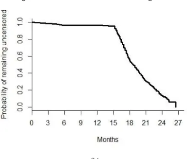
4. Set the study patients’ accrual period and follow-up time distribution, which depend on the practical limitations. Here, for illustration, assume we would have similar accrual and follow-up time patterns as those from CheckMate- 057. Figure 2 shows the censoring distribution by pooling the data from both treatment groups from CheckMate-057. Since the primary endpoint is OS time, we may assume that each patient’s mortality status was known at the end of the study. From Figure 2, it appears that the accrual time period was about 11 months, with patients entering the study uniformly over this time period, and the last patient enrolled was followed for 15 months. Under these assumptions, future patients who enter the potential trial in the first two months are expected to have at least 24 months of follow-up. Therefore, the RMST for each treatment group can be estimated well. Other

enrollment and follow-up patterns can be considered as well for designing a study. The key is to ensure that the potential follow-up time for a nontrivial proportion of patients is adequate for estimating the RMST in the specified time window.

Figure 4. Distribution of the Censoring Times

(36)

35

5. To estimate the sample size under the above setting, for any given sample size n with 1:1 treatment allocation, we generate a sample of OS times for each group using the above exponential distributions. We then generate corresponding censoring times via the distribution determined by the 11 months of accrual period and additional 16 months of follow-up after the completion of accrual. With these two samples of censored OS time data, the estimate of the difference in RMST, its variance estimate using pooled data from two treatment groups, and the corresponding test statistic, Z-score, are recorded. We repeat this simulation procedure, say, 3000 times, to

approximate the power of this potential study. If the power is less (or greater) than 90%, we then increase (or decrease) the sample size n and repeat the above process until the empirical power reaches the target level.

This results in a total of 336 patients (168 per arm) to obtain 90% power to detect a 3-month difference in RMST. Note that conventionally the

reciprocal of the average of the above 3000 variance estimates is coined as the total information time of the study. For the present case, the average standard error for the RMST difference estimate is about 0.94 months. With this standard error, the expected 95% CI would be about 1 – 5 months.

6. Like other clinical trials, when we apply a proposed design setting to conduct a real study, the patients’ accrual profile and follow-up time distribution are likely different from the assumed ones. For the present case, one may set the maximum calendar time for study termination being the time of the last patient entering the study plus 24 months. The study may be terminated early when the observed standard “information time”

(37)

36

(the reciprocal of variance estimate of the RMST difference) at a specific time point reaching the above total information time specified in Step 5. In fact, the trial may be terminated when, for instance, a handful of patients in each arm has reached 24 months of follow-up.

Note that when using the conventional log-rank test as the primary analysis tool, we set a specific total number of events as the total information time. To estimate the study sample size, we also need to assume the patients’

accrual/follow-up temporal profile. When the event rate is unexpectedly low in the real study, using such a total time information measure may unnecessarily prolong the study duration. On the other hand, with the t-year mean survival time difference or rate as the group contrast measure, the study would have a well-defined maximum duration time.

The procedure for designing a comparative trial with survival data discussed here can be implemented via the contributed R package SSRMST from the CRAN website (https://cran.r-project.org/web/packages/SSRMST/index.html).

(38)

37

3.4 Discussion

The design and analysis of a conventional cancer clinical trial with OS/PFS outcome can be improved by adopting a robust statistical procedure that enables clinically meaningful interpretation of the treatment effect. The RMST based statistical method may be used as a primary tool for design and analysis of a comparative study. It may also help us to better

understand the clinical interpretation of the HR when the proportional hazards model assumption is plausible. For the RMST or t-year mean survival time, the choice of t-year is a study characteristic, which should be pre-specified in the study protocol with a certain clinical justification. This time point should not be changed for the final primary analysis. The

exploratory analysis may be conducted with various time windows.

(39)

38

Chapter 4 Conclusion

In this thesis, the simulation results for the proposed monitoring tool showed that the tool does not affect size or power, but dramatically reduces the expected number of interim analyses when the effect of the treatment difference is small. The tool serves as a useful reference when interpreting the summary of the blinded data throughout the trial, without losing the integrity of the study. This tool could potentially save the study resources and budget by avoiding unnecessary interim analyses.

In addition, this thesis proposes the design using RMST, which is

statistically robust and clinically interpretable endpoint. The design and analysis of a conventional cancer clinical trial can be improved by adopting a robust statistical procedure that enables clinically meaningful

interpretations of the treatment effect. The RMST-based quantitative method may be used as a primary tool for future cancer trials or to help us to better understand the clinical interpretation of the HR even when its model assumption is plausible.

For clinical trial design, it is necessary to pre-specify the appropriate study endpoint and statistical analysis method in detail according to the clinical benefit of the targeted therapy and the population. Both proposals in this

(40)

39

thesis may be useful for future clinical trial design, and it is expected to be able to introduce study protocol that can overcome the existing challenges in clinical trials of cost/resource problems and interpretation of treatment effect from the statistical viewpoint. To improve the pharmaceutical

development process for clinically useful treatment, a pre-specified tool for decision making to consolidate cost/resource into the trials for beneficial treatment would be critical. It is also essential from the viewpoint of the social significance of clinical trials that statistical methods and the results obtained in clinical trials are useful and interpretable for clinicians and patients.

Generally, the primary goal of a comparative clinical study is to estimate an overall treatment effect. However, a “positive” trial based on such an

average effect over the entire patient population does not mean every patient would benefit from it. On the other hand, a “neutral or negative”

trial does not mean no patients would benefit from the new therapy. For designing future cancer studies, it is essential to have a pre-specified procedure based on the patients’ baseline characteristics collectively to identify a so-called high-value subgroup of patients who would clinically benefit from the new therapy.²⁴ In published guidance on the enrichment strategies for clinical trials,²⁵ the US FDA encourages the clinical trialists to consider such a predictive enrichment strategy. This pre-specified procedure would be an ideal tool to identify, and future work will examine the design to identify future patients to be treated by targeted therapy. For example, a specific subgroup of patients who would benefit from nivolumab or

(41)

40

pembrolizumab for treating a specific subpopulation of NSCLC patients via trials such as CheckMate-057, CheckMate-026²⁶ and KeyNote-024 with the patient’s baseline information regarding, for instance, PD-L1, gene

signatures and epitope load et al collectively.

(42)

41

References

1. Ellenberg SS, Fleming TR, DeMets DL. Data monitoring committees in clinical trials: a practical perspective. Chichester: John Wiley & Sons, 2002.

2. International Conference on Harmonization (ICH). Guidance for Industry:

E9 statistical principles for clinical trials. Rockville, MD: Food and Drug Administrations; September 1998.

3. Ball G. Continuous safety monitoring for randomized controlled clinical trials with blinded treatment information; Part 4: One method. Contemp Clin Trials 2011; 32: S11-S17.

4. Wen S, Ball G, and Dey J. Bayesian monitoring of safety signals in blinded clinical trial data. Ann Public Health Res 2015; 2(2): 1019.

5. Yao B, Zhu L, Jiang Q, and H. Amy Xia. Safety monitoring in clinical trials. Pharmaceutics 2013; (5): 94-106.

6. Thall PF, Simon R. Practical Bayesian guidelines for phase IIB clinical trials. Biometrics 1994; 50(2): 337-49.

7. Lan KKG and DeMets DL. Discrete sequential boundaries for clinical trials. Biometrika 1983; 70(3): 659-663.

8. Jennison C and Turnbull BW. Group Sequential Methods with Applications to Clinical Trials. Chichester: John Wiley & Sons, 2000.

9. Haybittle JL. Repeated assessment of results in clinical trials of cancer treatment. Br J Radiology 1971; (44): 93–797.

10. Peto R, Pike MC, et al. Design and analysis of randomized clinical trials requiring prolonged observation of each patient: Part I. Introduction and Design. Br J Cancer 1976; (34): 585–612.

(43)

42

11. Rajkumar SV, Blood E, Vesole D, Fonseca R, Greipp PR. Phase III clinical trial of thalidomide plus dexamethasone compared with

dexamethasone alone in newly diagnosed multiple myeloma: A Clinical Trial Coordinated by the Eastern Cooperative Oncology Group. J Clin Oncol 2006;

24(3): 431-436.

12. Uno H, Claggett B, Tian L, et al. Moving beyond the hazard ratio in quantifying the between-group difference in survival analysis. J Clin Oncol 2014; 32:2380-5.

13. Uno H, Wittes J, Fu H, et al. Alternatives to hazard ratios for comparing the efficacy or safety of therapies in noninferiority studies. Ann Intern Med 2015; 163:127-34.

14. Péron J, Roy P, Ozenne B, et al. The net chance of a longer survival as a patient-oriented measure of treatment benefit in randomized clinical trials.

JAMA Oncol 2016; 2:901-905.

15. Chappell R, Zhu X. Describing Differences in Survival Curves. JAMA Oncol 2016; 2:906-907.

16. Trinquart L, Jacot J, Conner SC, et al. Comparison of treatment effects measured by the hazard ratio and by the ratio of restricted mean survival times in oncology randomized controlled trials. J Clin Oncol 2016; 34:1813-9.

17. A’Hern RP. Restricted mean survival time: An obligatory end point for time-to-event analysis in cancer trials? J Clin Oncol 2016; 34:3474-6.

18. Cox DR. Regression models and life tables. J R Sat Soc B. 1972; 34:187- 220.

19. Reid N. A conversation with Sir David Cox. Statistical Science 1994;

(44)

43

9:439-55.

20. Royston P, Parmar MKB. Restricted mean survival time: an alternative to the hazard ratio for the design and analysis of randomized trials with a time-to-event outcome. BMC Med Res Methodol2013; 13(1), 152.

21. Borghaei H, Paz-Ares L, Horn L, et al. Nivolumab versus docetaxel in advanced nonsquamous non–small-cell lung cancer. N Engl J Med 2015;

373:1627-39.

22. Guyot P, Ades AE, Ouwens MJ, Welton NJ. Enhanced secondary analysis of survival data: reconstructing the data from published Kaplan-Meier survival curves. BMC Med Res Methodol 2012; 12:9.

23. Parzen MI, Wei LJ, Ying Z. A resampling method based on pivotal estimating functions. Biometrika 1994; 81:341-50.

24. Li J, Zhao L, Tian L, et al. A predictive enrichment procedure to identify potential responders to a new therapy for randomized, comparative controlled clinical studies. Biometrics 2016; 72:877-87.

25. U.S. Food and Drug Administration. Guidance for industry: Enrichment strategies for clinical trials to support approval of human drugs and biological products, 2012.

26. Socinski M, Creelan B, Horn L, et al. NSCLC, metastatic CheckMate 026:

A phase 3 trial of nivolumab vs investigator's choice (IC) of platinum-based doublet chemotherapy (PT-DC) as first-line therapy for stage iv/recurrent programmed death ligand 1 (PD-L1)-positive NSCLC. Ann Oncol 27, 2016 (suppl 6).

Statistical considerations for design and analysis of comparative clinical trials