Hideyasu Shimadzu
March 2008
Preface
Far better an approximate answer to the right question, which is often vague, than an exact answer to the wrong question, which can always be made precise.
(The future of data analysis,Annals of Mathematical Statistics33:1-67, 1962)
— John W. Tukey Modelling is a fundamental of Science. It is of much importance to create a model which leads people to many discoveries. A better model can be constructed in a framework which better captures the reality. The Data modelling starts from establishment of such a framework by honestly looking at the observed data.
Biological data modelling is somewhat specific because the variability of data remains significant even if the experiment were carefully designed. It is nothing more than the sign of alive that homoeostasis or constancy is maintained in any of biological phenomena. It is also often the case when biological data is obtained only once as a function of time. The aim of this thesis to seek for possible ways to a good biological data modelling, which will be suggested by three case studies.
The first case study is on modelling five bird count series observed monthly. Each of the series was decomposed into three components: long trend, short trend and irregular by two step smoothing. It was clearly shown that a simple linear transformation of the long trends as a whole
i
is a good modelling for capturing relationships between bird count series and environmental changes. It turned out that there are two bird groups, one of which increases in number as an increase of resident area and the other decreases as a decrease of farmland area. Each short trend also allows us to understand the seasonality of the behaviour of each bird.
The second case study is on modelling swimmers’ speeds over the course of a male 200 m free-style race. The model is based on a dynamical model reflecting the trade–off between drag and propulsion in swimming. It does not only fit well the data but also provide a good description of the swimming strategies of each swimmer from phase to phase in the race. An individual factor measuring how much faster or slower the individual swims relative to the average swimming speed is estimated. This factor is, as expected, closely related to the final outcome of the race.
The third case study is on modelling membrane potential of a neuron.
A simple but powerful input and output system has been created by noting that each nerve cell system has two different type of synapses; chemical and electrical ones. Three phase model has been introduced for the input as well as for the spikes, which is a simplified Hodgkin–Huxley model but with an extra phase, pre–activation phase. Spike occurrences are modelled by a point process with the intensity proportional to the derivative of the input. The model would be applicable for any other membrane potential changes of a neuron as an integrated model.
An important implication of these case studies is that the models created are not a simple extension of existing theories or models. Such models could not be obtained without careful analysis of the given data. Honest approach to the data was a key to success. As a summary, it is shown that
data–driven approach is likely to open a new horizon particularly in biological data modelling because an innovative modelling is always necessary to cope with the large variability of the data.
Acknowledgements
I would like to express my sincerest gratitude to my supervisor, Professor Ritei Shibata for his patient guidance and encouragement. This thesis could not have been accomplished without his support. His profound insights and enthusiasm for researches are exceptional. It is my privilege to have met his philosophy of Data Science earlier on.
I would also like to express my thank to Professors Makoto Maejima, Yuji Ohgi, Kotaro Oka, Kunio Shimizu for their comments and suggestions on the earlier version of this thesis, which are very helpful to improve it.
The researches presented in this thesis have been investigated as joint research with people in each area, without whom these would not have been completed. Especially, the bird census data was provided from Jiyu–Gakuen where I graduated, the swim race data was from the Medicine and Scientific Committee of Japan Swimming Federation and the neural action potential data was from Mr Toshinobu Shimoi (Keio University). I would like to thank these groups and people for their contributions and kind approve to analyse these data sets.
During my studies, there are many people had the misfortune of crossing my path and having to spend time for me. Dr Matthew Browne (the Commonwealth Scientific and Industrial Research Organisation Mathematical and Information Sciences, Australia) was my host during my
iv
visit to CSIRO Cleveland laboratory, from October to November 2007. Many discussions with him was great help to get new ideas in my research. Professor Ryozo Miura (Hitotsubashi University) was an adjunct lecturer in Statistics when I was an undergraduate student. He taught me a fascination of data analysis and gave me a motivation to enter this area. Dr Peter Thomson (Statistics Research Associates Limited, New Zealand) is a member of the advisory board for the 21st Century Centre of Excellence (COE) Programme:
Integrative Mathematical Sciencesat Keio University. Many discussions with him in tea time and seminars during his annual visit to Keio University were substantially improved my researches. I am very grateful to these people for their kind support and encouragement.
Thanks all are due to everyone else who has given me many help and support during my studies at Keio University, especially the member of Shibata Laboratory including Dr Natsuhiko Kumasaka and Mr Yuki Sugaya.
Financial support, over my PhD studies, from COE Programme is gratefully acknowledged.
March 2008 Hideyasu Shimadzu
Contents
Preface i
Acknowledgements iv
1 Introduction 1
1.1 Biological data . . . . 1
1.2 Modelling . . . . 2
1.2.1 Modelling process . . . . 2
1.2.2 Data and mechanism behind . . . . 3
1.2.3 Complexity and accuracy of the model . . . . 3
1.3 Smoothing technique: loess . . . . 4
2 Bird count series modelling 6 2.1 Introduction . . . . 6
2.2 Bird census . . . . 7
2.3 Data . . . . 8
2.3.1 Natural environment of observational place . . . . 8
2.3.2 Data collection . . . . 8
2.3.3 Target species . . . . 10
2.4 Time series decomposition through loess . . . . 13
vi
2.5 Relationships between bird count series and environmental
factors . . . . 15
2.5.1 Long trend . . . . 18
2.5.2 Short trend . . . . 23
2.5.3 Irregular series . . . . 27
2.6 Summary . . . . 28
3 Swimmers’ speeds modelling 31 3.1 Introduction . . . . 31
3.2 Data . . . . 33
3.3 Model . . . . 34
3.3.1 An underpinning deterministic model . . . . 34
3.3.2 A stochastic model for swimming speed . . . . 38
3.4 Result . . . . 40
3.4.1 Common swimming speed and its parameters . . . . . 40
3.4.2 Individual parameters . . . . 42
3.4.3 Discussion . . . . 43
3.5 Summary . . . . 47
4 Membrane potential modelling 48 4.1 Introduction . . . . 48
4.2 Data . . . . 49
4.2.1 Data collection . . . . 49
4.2.2 Data exploration . . . . 50
4.3 Model . . . . 51
4.3.1 Model for spikes . . . . 52
4.3.2 Model for the input . . . . 55
4.4 Model identification . . . . 56
4.4.1 Identification of the spike model . . . . 56
4.4.2 Identification of the input model . . . . 57
4.4.3 Results of simulation . . . . 60
4.4.4 Identification of the intensity for the occurrence time of spikes . . . . 61
4.5 Summary . . . . 65
5 Conclusion 66
Chapter 1 Introduction
1.1 Biological data
Biological data is the data collected from biologicals sources, whose variability remain lage even if experiments were carefully organised. It is nothing more than the sign of alive but can be a burden of biological data modelling. Specific features of biological data indispensable in the modelling are Homoeostasis (Constancy), Uncontrollable observation and Time dependency. In the subsequent sections, we concentrate our attention into the following three biological data.
1. Bird count data (Bird);
2. Swimming race data (Human);
3. Neural membrane potential data (Neuron).
Table 1.1 summarises the specific features of those three data sets. Most important feature would be the constancy, in other words, the homogeneity of the data is retained in a group of birds, in each phase of swimming races and membrane potential changes by focusing on the constancy. This suggests that a better modelling approach is, as a first step, to construct a model only
1
Table 1.1: Specific features of the data dealt in this thesis.
Bird Human Neuron
Homoeostasis Environment Race Ion
Constancy Group Phase Phase
Uncontrollable Open system Competition In vivo
Observation Once Once Once
Time dependency Yes Yes Yes
for such data sets holding true for constancy since the model built might be simple and easily interpreted.
1.2 Modelling
1.2.1 Modelling process
There is no definite way of biological data modelling but there are two basic principles which any data scientist should observe, although those are quite general and applicable for any scientific data modelling. The first principle is ”Be honest to the given data” and the second one is ”Keep a good relation to the scientist in the field”. The latter makes possible to discuss what is the target of modelling and how to approach the problem. Sometimes it results in re-sampling or re-experiments.
In the process of modelling, preliminary analysis of the data is also important. Only a good preliminary analysis can provide a successful model which fits the data well and gives good explanation. It is often the case when it results in coming back to the first stage, the data collection stage. The value of modelling is, of course, how large the impact is of the model created to the field of science. New discovery or constructive suggestion is modes most desirable as a result of the modelling.
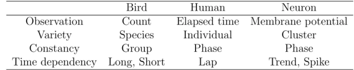
Table 1.2: Fundamental aspects of the data.
Bird Human Neuron
Observation Count Elapsed time Membrane potential
Variety Species Individual Cluster
Constancy Group Phase Phase
Time dependency Long, Short Lap Trend, Spike
1.2.2 Data and mechanism behind
In the stage of preliminary analysis, a crucial point is to grasp various aspects of the data in an appropriate manner. Table 1.2 summarises fundamental aspects of the data employed in the three case studies. Correct understanding of the aspects leads people to correct modelling, although it is not enough. As was mentioned, the constancy may suggest a framework for better modelling.
Is is also necessary to consider whether it could be able to ignore the difference between individual.
Furthermore, it is also of importance to capture the mechanism behind the data for successful modelling. It can be achieved only by continuous discussion with the scientists in the underlying research field. In the case of physics, such well known structures have been given by differential equations.
However, such models show sometimes different behaviour from the data observed. This suggests that the assumptions for such model may not be true and the model need to be improved.
1.2.3 Complexity and accuracy of the model
Modelling is an endless work. A well known principle of modelling is to make a good balance between the complexity and accuracy of modelling (Akaike, 1973, Konishi and Kitagawa, 1996, 2007). In other word, parsimonious model
is most desirable. But there is always room for improvement of the model created. Efforts to improve the model is necessary, but time and data are limited. A criterion for the stop of our effort would be if the model has reflected all necessary information in the data.
1.3 Smoothing technique: loess
Smoothing techniques are of use to extract structures lying behind data, especially, if any significant structure cannot be assumed. There is a useful technique called local polynomial regression proposed by Cleveland (1979), Cleveland and Devlin (1988) which is available on S–PLUS as a function lowess orloess.
Local polynomial regression assumes a smooth function f(x), as an expected structure, behind data (xi, yi), i = 1,2, . . . , n, which are observed and locally approximate using polynomials. The weight used for weighted least squared method for estimation is
∑n i=1
w
(|xi−x| dδ(x)
)
{yi−fx(xi)}2 →
fx
min, (1.1)
where
dδ(x) = max
i;xi∈Uδ(x)|xi−x|.
Here Uδ(x) is the nearest neighbour of x defined by [nδ], which is the maximum integer ofnδ. The smoothing parameterδmeans the proportion of observations in the nearest neighbour. Further, fx is a p–degree polynomial given by
fx(z) =
∑p k=0
βk(x) (z−x)k.
The weight function w for weighted least squared in S–PLUS is a tori cubic weight
w(x) =
(1−x3)3 (0≤x <1), 0 (otherwise). Introduce some matrix notations, for convenience. Put X(x) =
1 (x1−x) · · · (x1−x)p ... ... . .. ... 1 (xn−x) · · · (xn−x)p
, βˆ(x) =
βˆ0(x) ... βˆp(x)
,
W (x) = diag [
w
(x1−x dδ(x)
)
,· · ·, w
(xn−x dδ(x)
)]
, y=
y1
... yn
.
X(x) is ann×(p+ 1) design matrix andW(x) is ann×ndiagonal matrix of weights.
The solution of the least squares problem can be written as βˆ(x) =A−1(x)XT(x)W (x)y ,
where
A(x) =XT (x)W (x)X(x) .
A(x) ={am,r(x)} is the (p+ 1)×(p+ 1) symmetric matrix and its (m, r) element is written as
am,r(x) =
∑n i=1
(xi−x)m+r−2w
(xi−x dδ(x)
)
. (1.2)
The smoothed value atx is given by βˆ0(x) = 1
detA(x)
∑p k=0
adj (A(x))1,k+1
∑n i=1
(xi−x)kw
(xi−x dδ(x)
)
yi , (1.3) where adj (A(x))1,k+1 is the cofactor of ak+1,1(x).
This technique will be used in Section 2 and 4 for extracting some structures which could not assume any mechanisms behind the data.
Chapter 2
Bird count series modelling to explore environmental changes
2.1 Introduction
Relationships between avifauna and natural environment have been attracting many researchers’ interests in ecology. However, their interests have been rather biased to abundance of species, particularly in field studies conducted in Japan, see Higuchi et al. (1982), Anada and Fujimaki (1984), Hirano et al. (1985, 1989), Murai and Higuchi (1988), Kurosawa (1994), Ootaka and Nakamura (1996) and Maeda (1998). Although frequency changes of each species would be of much importance to capture the effects of human activities which are apt to cause environmental changes for birds, not so many works have been done on the number of birds observed in an area for each species but there are several papers, Hirano (1996), Komeda and Ueki (2002), Uchida et al. (2003), Shimadzu and Shibata (2005).
In this chapter, the data observed over 35 years at Jiyu–Gakuen in Tokyo, Japan, is used to explore relationships between the number of individuals and environmental changes due to human activities. The data has been collected monthly in a well organised way. By two step smoothing technique, each bird
6
count series is decomposed into three components,long trend,short trendand irregular. To explorer relationships between those long trends and several environment indices, the scale and location of each long trend is adjusted.
As a consequence, two bird groups are popped up. One is the group of Turtle Dove (Streptopelia orientalis), Brown–eared Bulbul (Hypsipetes amaurotis) and Great Tit (Parus major) and the adjusted long trends all fit well to the curve of increasing residential area. Another is the group of Tree Sparrow (Passer montanus) and Gray Starling (Sturnus cineraceus) and the adjusted long trends all fit well to the curve of decreasing farmland area. It will be shown that each short trend provides significant information on the seasonal behaviour of each species.
2.2 Bird census
There have been various bird censuses conducted but not necessarily well organised. Its objective, the period or the method varies census by census.
Census by a national institution is usually well organised and the data is open to public on the web. Two examples of such censuses are Common Bird Census (CBC;http://www.bto.org/index.htm) conducted by British Trust for Ornithology (BTO) over the whole of the United Kingdom since 1962, and Breeding Bird Survey (BBS; http://www.mp2-pwrc.usgs.gov/bbs/) conducted by the United States Geological Survey (USGS) and the Canadian Wildlife Service (CWS) since 1966.
On the other hand, bird censuses in Japan are usually conducted by individuals or small groups, so that the collected data are not necessarily open to public but scattered over individuals or groups in Japan. In this respect, the data collected at Jiyu–Gakuen is valuable because it is the result
of a continuous survey of the number of birds in a fixed area over 35 years and the data is open to public as is explained later.
2.3 Data
2.3.1 Natural environment of observational place
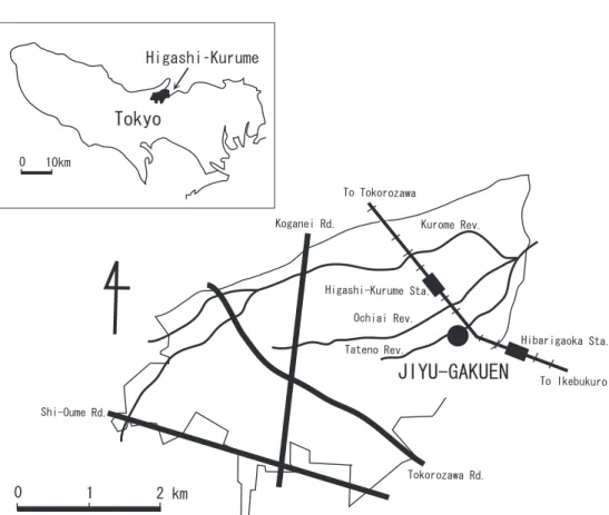
Higashi–Kurume city where Jiyu–Gakuen is located is 20 km far from the centre of Tokyo and on the centre of Musashino plateau on the loamy layer of Kanto. She covers 12.92 km2 area lying 6.5 km east and west, 3.5 km south and north and has three rivers crossing to the east: the Kurome River, Ochiai River and Tateno River.
Jiyu–Gakuen campus is located on the southeast end of Higashi–Kurume city as is shown in Figure 2.1 and covers 100,000 m2. Many trees and bushes are found in the campus, for example, Japanese maple (Acer palmatum), Japanese zelkova (Zelkova serrata), Ginkgo (Ginkgo biloba), Korean hornbeam (Carpinus tschonoskii), Red pine (Pinus densiflora), Japanese white oak (Quercus myrsinaefolia), and Japanese aucuba (Aucuba japonica). Also farm place, glass land and several ponds can be found in the campus.
2.3.2 Data collection
Once a month, the census is conducted by about 40 students of the secondly school and the number of birds for each species are recorded. Whole area of the campus is investigated before noon (about 30 min between 9 to 11 am) of a fine day with no rain and light wind.
Various types of bird census have been conducted (Bibbyet al., 2000). For example, Territory mapping used in CBC is the census to identify territory
*KDCTKICQMC5VC
*KICUJK-WTWOG5VC 1EJKCK4GX
-WTQOG4GX -QICPGK4F
6QMQTQ\CYC4F 5JK1WOG4F
MO
0 10km
Tokyo
Higashi‑Kurume
,+;7)#-7'0
6CVGPQ4GX
6Q+MGDWMWTQ 6Q6QMQTQ\CYC
Figure 2.1: Jiyu–Gakuen in Tokyo, Japan.
of each bird and Point counts used in BBS or Line transectsfrequently used in Japan is the census to know the number of birds in an area. Line transects is advantageous in mountainous area. Although census has to be carefully designed depending on target species, environment conditions and quality of participants to the survey, complete sampling is adopted in this survey because of the quality of participants (Kira, 2000).
The data observed is available from Kiraet al. (2002) or on the web
http://www.stat.math.keio.ac.jp/DandDIII/Examples/JiyuBirdCount.dad
which is organised along with the DandD (Data and Description) rule (Shibata, 2001, Yokouchi and Shibata, 2001).
2.3.3 Target species
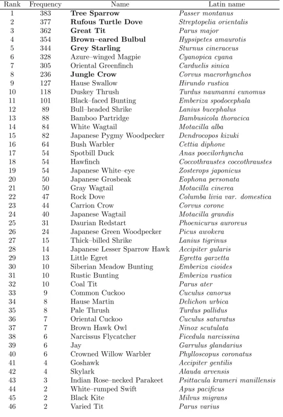
More than 60 species have been observed for 32 years from 1967 to 1998, but some of them are not frequently observed as is seen on Table 2.1. In this chapter, only eight species out of 60 species are taken into consideration.
In those eight species, Azure–winged Magpie and Oriental Greenfinch are exceptional. As is seen in the count series shown in Figure 2.2, the count series of each species does not show any clear trend but rather oscillating. The reason is not the same for those two species. Oriental Greenfinch is a winter visitor of which the number largely depends on richness of foods (seeds of grass and trees) during autumn to winter. On the other hand, Azure–winged Magpie is usually moving within small bevy so that, the observed number can be large if the census were organised during their occasional visit.
Table 2.1: Observed frequency of birds for each species.
Rank Frequency Name Latin name
1 383 Tree Sparrow Passer montanus
2 377 Rufous Turtle Dove Streptopelia orientalis
3 362 Great Tit Parus major
4 354 Brown–eared Bulbul Hypsipetes amaurotis 5 344 Grey Starling Sturnus cineraceus
6 328 Azure–winged Magpie Cyanopica cyana
7 305 Oriental Greenfinch Carduelis sinica
8 236 Jungle Crow Corvus macrorhynchos
9 127 Hause Swallow Hirundo rustica
10 118 Duskey Thrush Turdus naumanni eunomus
11 101 Black–faced Bunting Emberiza spodocephala
12 89 Bull–headed Shrike Lanius bucephalus
13 88 Bamboo Partridge Bambusicola thoracica
14 84 White Wagtail Motacilla alba
15 82 Japanese Pygmy Woodpecker Dendrocopos kizuki
16 64 Bush Warbler Cettia diphone
17 54 Spotbill Duck Anas poecilorhyncha
18 54 Hawfinch Coccothraustes coccothraustes
19 54 Japanese White–eye Zosterops japonicus
20 50 Japanese Grosbeak Eophona personata
21 50 Gray Wagtail Motacilla cinerea
22 47 Rock Dove Columba livia var. domestica
23 44 Carrion Crow Corvus corone
24 40 Japanese Wagtail Motacilla grandis
25 31 Daurian Redstart Phoenicurus auroreus
26 24 Japanese Green Woodpecker Picus awokera 27 15 Thick–billed Shrike Lanius tigrinus 28 14 Japanese Lesser Sparrow Hawk Accipiter gularis
29 13 Little Egret Egretta garzetta
30 10 Siberian Meadow Bunting Emberiza cioides
31 10 Rustic Bunting Emberiza rustica
32 10 Coal Tit Parus ater
33 9 Common Cuckoo Cuculus canorus
34 8 Hause Martin Delichon urbica
35 8 Pale Thrush Turdus pallidus
36 7 Oriental Cuckoo Cuculus saturatus
37 7 Brown Hawk Owl Ninox scutulata
38 6 Narcissus Flycatcher Ficedula narcissina
39 6 Jay Garrulus glandarius
40 6 Crowned Willow Warbler Phylloscopus coronatus
41 4 Goshawk Accipiter gentilis
42 4 Skylark Alauda arvensis
43 3 Indian Rose–necked Parakeet Psittacula krameri manillensis
44 2 White–rumped Swift Apus pacificus
45 2 Black Kite Milvus migrans
46 2 Varied Tit Parus varius
47 2 Ashy Minivet Pericrocotus divaricatus
48 2 Siberian Bluechat Tarsiger cyanurus
49 2 Brown Thrush Turdus chrysolaus
50 2 Naumann’s Thrush Turdus naumanni naumanni
51 1 Teal Anas crecca
52 1 Indian Tree Pipit Anthus hodgsoni
53 1 Jungle Nightjar Caprimulgus indicus
54 1 Blue–and–white Flycatcher Cyanoptila cyanomelana 55 1 Red–breasted Flycatcher Ficedula parva
56 1 Black–headed Gull Larus ridibundus
57 1 Grey–spotted Flycatcher Muscicapa griseisticta
58 1 Night Heron Nycticorax nycticorax
59 1 Honey Buzzard Pernis apivorus
60 1 White’s Ground Thrush Zoothera dauma
Oriental Greenfinch (Carduelis sinica)
1966 1968 1970 1972 1974 1976 1978 1980 1982 1984 1986 1988 1990 1992 1994 1996 1998 2000
04080120160200
Azure-winged Magpie (Cyanopica cyana)
1966 1968 1970 1972 1974 1976 1978 1980 1982 1984 1986 1988 1990 1992 1994 1996 1998 2000
010305070(individual)
Figure 2.2: Count series of Oriental Greenfinch and Azure–winged Magpie.
The target species are now six species; Turtle Dove,Brown–eared Bulbul,Great Tit,Tree Sparrow,Gray Starling and Jungle Crow, which are indicated by bold font on Table 2.1. As a consequence, those are the species categorised into resident bird being observed over year in this area.
It is naturally expected that their number of such a bird is strongly related with environmental changes.
2.4 Time series decomposition through loess
In time series analysis, seasonal adjustment has been widely used to extract seasonal movements. The expectation is to find a seasonal structure lying behind the data. Particularly in economics, considered are yearly, monthly or weekly seasonalities. However, in terms of birds, weekly or monthly seasonality would not be reasonable. Even if there were yearly seasonality,
it would not be so exact as in economical time series. Therefore, two step smoothing technique will be employed in place of seasonal adjustment, to decompose the original time series into three components.
There are two typical smoothing techniques:
• Spline smoothing;
• Local polynomial regression.
Spline smoothing fits a piecewise polynomial function to the given data, where the pieces are specified by the given knots. It is assumed that the derivatives of the function are continuous up to an order. On the other hand, local polynomial regression provides the smoothed value by fitting a polynomial by weighted regression in a neighbourhood of each target point.
Kernel smoothing is a variant of local polynomial regression where the order of polynomials is zero. An implementation of the local polynomial regression is loess by Cleveland (Cleveland, 1979, Cleveland and Devlin, 1988) which is available on S–PLUS. There are good examples and detailed discussions on polynomial regression modelling in Chambers and Hastie (1992) or Fan and Gijbels (1996). Several works have been done for bird count series to find relation to environmental conditions by using such a local polynomial regression technique. For example, James et al. (1996) applied the technique to BBS data for 26 years from 1966 to 1992 and analysed 26 species of American Warblers observed in the central America. Their main result is that the number of birds largely depends on the altitude of observational place, but also they found that the deterioration of food environment by air pollution as a cause of possible.
Here it is assumed that the original series Zi(t) of species i can be
decomposed into two components and noise as
Zi(t) =Li(t) +Si(t) +Ii(t) (t= 1, . . . ,384).
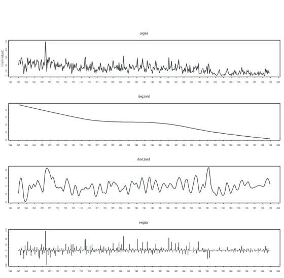
where Li(t) is long trend which behaves slow in decade–long span, Si(t) is short trend having yearly span and Ii(t) is irregular. The long trend Li(t) is extracted by applying smoothing technique loess to the original series Zi(t). Further, the short trendSi(t) is extracted from Zi(t)−Li(t) by the same way with shorter span. Such decomposition approach called two step smoothing was applied for a financial time series (Shibata and Miura, 1997).
An example of the decomposition for Tree Sparrow is shown in Figure 2.3.
The top panel is the original series Zi(t) and the bottoms are following the order, long trend Li(t), short trendSi(t) and irregular Ii(t).
Without any assumption of specific cycles, local polynomial regression provides smoothing values. This is desirable aspects if it is not able to assume any structure behind the data. It is necessary to chose a smoothing parameter δ by span and a degree of polynomial p by degree in S–PLUS. There are several discussions on selection of these parameters (Fan and Gijbels, 1996).
However it is important how extract a reasonable trend which can be easily interpreted. Choice of parameters will be discussed in following.
2.5 Relationships between bird count series and environmental factors
Applying such smoothing technique to each of six species listed in Section 2.3.3 to extract long trend, it was clearly shown that those species are categorised into two groups, one of which increases and another decreases.
Turtle Dove, Great Tit, Brown–eared Bulbul and Jungle Crow are included
1966 1967 1968 1969 1970 1971 1972 1973 1974 1975 1976 1977 1978 1979 1980 1981 1982 1983 1984 1985 1986 1987 1988 1989 1990 1991 1992 1993 1994 1995 1996 1997 1998 1999 2000
04080140200260
original
1966 1967 1968 1969 1970 1971 1972 1973 1974 1975 1976 1977 1978 1979 1980 1981 1982 1983 1984 1985 1986 1987 1988 1989 1990 1991 1992 1993 1994 1995 1996 1997 1998 1999 2000
1030507090
long.trend
1966 1967 1968 1969 1970 1971 1972 1973 1974 1975 1976 1977 1978 1979 1980 1981 1982 1983 1984 1985 1986 1987 1988 1989 1990 1991 1992 1993 1994 1995 1996 1997 1998 1999 2000
-40-2002040
short.trend
1966 1967 1968 1969 1970 1971 1972 1973 1974 1975 1976 1977 1978 1979 1980 1981 1982 1983 1984 1985 1986 1987 1988 1989 1990 1991 1992 1993 1994 1995 1996 1997 1998 1999 2000
-100-4004080140
irregular
(individual)
Figure 2.3: Count series decomposition of Tree Sparrow.
1966 1969 1972 1975 1978 1981 1984 1987 1990 1993 1996 1999
0123456789(individual)
Figure 2.4: The long trend of Jungle Crow.
into the former group and Tree Sparrow and Gray Starling are included into the latter group. As to Jungle Crow, it is also increasing, but Figure 2.4 shows the different increase competitive of Figure 2.6. Such increase of Jungle Crow has been recently reported especially in urban areas over Japan. There are several causes possible, for example, the growth of trees. It would not be appropriate to discuss this species same as other so it will be dropped from the target and leave this for the future. For instance, only five species; Turtle Dove, Brown–eared Bulbul, Great Tit, Tree Sparrow and Gray Starling are analysed.
The long trends extracted from each count series are compared with environmental factors to find any clear relationships between them. Although there are, as candidates, several environmental factors, temperature, the area of classification of land, for example. It is consequently found that
four environmental factors of Higashi–Kurume city which may have strong relationships with the number of individuals:
• Resident area [km2], increase;
• Farmland [km2], decrease;
• Length of paved road [km], increase;
• Length of unpaved road [km], decrease.
These four factors are, as expected, related each other. However, such relations are not specific.
It would be the easiest way to overlay these two different time series having different scale. So a linear transformation is adopted for the long trend of each species to adjust their scale parameteraiand location parameterbias close as possible to each environmental factor; the area of farmland F (t) or the resident areaR(t). The parameters are defined by least squared method,
∑384 t=1
{F (t)−(aiLi(t) +bi)}2 −→
ai,bi
min (i= 1,2),
∑384 t=1
{R(t)−(aiLi(t) +bi)}2 −→
ai,bi
min (i= 3,4,5).
(2.1)
It is interesting to note that smoothing parameter δ for the long trend can be re–estimated so as to minimise the squared error simultaneously with the location and scale parameters. Such re–estimated smoothing parameters will be given in the next section.
2.5.1 Long trend
The estimated parameters (δ, ai, bi) which minimise the least squared error (2.1) are estimated with the degree of polynomial p = 1. The parameters
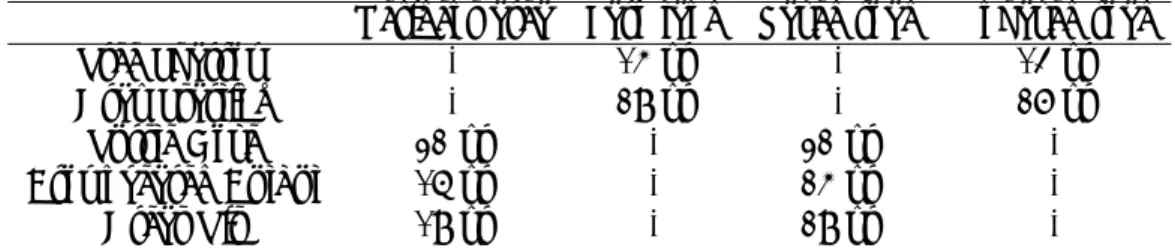
Table 2.2: Estimated smoothing parameter (span).
Resident area Farmland Paved road Unpaved road
Tree Sparrow - 15 yr - 14 yr
Gray Starling - 29 yr - 27 yr
Turtle Dove 32 yr - 32 yr -
Brown–eared Bulbul 16 yr - 25 yr -
Great Tit 19 yr - 29 yr -
Table 2.3: Estimated parameters adjust to resident area and farmland.
Resident area Farmland
ai bi ai bi
1 Tree Sparrow - - 0.038 1.215
2 Gray Starling - - 0.116 1.167
3 Turtle Dove 0.478 −0.638 - -
4 Brown–eared Bulbul 0.461 −0.028 - -
5 Great Tit 0.876 −0.417 - -
are shown in Table 2.2, 2.3, and 2.4. Attention to the increase of decrease of each time series, it is easily understand which environmental factor should be related with the bird count series. So then the parameters of those 3 species, Turtle Dove,Great Tit and Brown–eared Bulbul showing a increase trend are adjusted as close as possible to the resident area or the length of paved road in Higashi–Kurume city. The other hand, the rest of species;
Tree Sparrow and Gray Starling are adjusted to the area of farmland and the length of unpaved road. Un estimated parameters are indicated by ”-”.
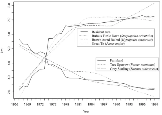
Figure 2.6 and 2.5 show the transformed long trends using parameters (Table 2.3, 2.4) and environment factors. These figures show that the long trends all are quite similar with environment changes, which means that the estimated parameters are significant. This show that the smoothing
Table 2.4: Estimated parameters adjust to the length of paved or unpaved road.
Paved road Unpaved road
ai bi ai bi
1 Tree Sparrow - - 1467.282 −32246.85
2 Gray Starling - - 4613.627 −36988.11
3 Turtle Dove 18405.29 −114019.4 - -
4 Brown–eared Bulbul 17448.08 −86633.47 - -
5 Great Tit 31743.47 −91209.35 - -
parameter chosen as p= 1 was enough, as well.
The estimated parameters for the three species; Turtle Dove, Brown–eared Bulbul and Great Tit in Table 2.4 take larger value than those of Table 2.3. This is because of the discontinuous behaviour of the length of paved road in Higashi–Kurume city. However, as is shown in Figure 2.6 and 2.5, their long trends show quite similar behaviour with referred environment changes even those having quite different properties. There is lying behind that the scenario of urbanisation would be considered. In fact, such rapid increase of resident area and decrease of farmland led by the high economic growth period in Japan. It is clearly shown that the resident area was lager than the farmland even since 1974.
These consideration naturally lead that the essential environmental factors for bird may be the change of resident area and farmland. Such close relationships between birds and the length of paved or unpaved road would be coincidence. It is not sure whether such significant relationship can be found from the observations in other place. This result implies the highly adaptability of birds to environment.
The two groups in Figure 2.5 can be well explained from the view
Year
km2
1966 1969 1972 1975 1978 1981 1984 1987 1990 1993 1996 1999
2.03.04.05.06.07.08.0
Resident area
Rufous Turtle Dove (Streptopelia orientalis) Brown-eared Bulbul (Hypsipetes amaurotis) Great Tit (Parus major)
Farmland
Tree Sparrow (Passer montanus) Grey Starling (Sturnus cineraceus)
Figure 2.5: The long trends and changes of resident area and farmland in Higashi–Kurume city.
Table 2.5: Ecological characteristics of each species.
Feeding Nesting Tree Sparrow Open land Open forest Gray Starling Open land Open forest
Turtle Dove Open forest Forest Brown–eared Bulbul Forest Forest
Great Tit Forest Forest
Year
km
1966 1969 1972 1975 1978 1981 1984 1987 1990 1993 1996 1999
-202060100140200
Paved road
Rufous Turtle Dove (Streptopelia orientalis) Brown-eared Bulbul (Hypsipetes amaurotis) Great Tit (Parus major)
Unpaved road
Tree Sparrow (Passer montanus) Grey Starling (Sturnus cineraceus)
Figure 2.6: The long trends and changes of the length of paved or unpaved road in Higashi–Kurume city.
point of ecological theory, the preference of environmental conditions of each species. Such preference of environmental characteristics of each species are summarised in Table 2.5. The increase of resident area leads the increase of garden plants and shade trees which make small green island. As a consequence, Turtle Dove, Brown–eared Bulbul and Great Tit which can adopt by themselves are increase. On the other hand, Tree Sparrow and Gray Starling which feed on farmland decreased. That is, the decrease of Tree Sparrow and Gray Starling were largely depending on the condition of feeding place.
2.5.2 Short trend
On decomposition of bird count series,middle trendwas possible to take into consideration. However, it was not significant because of its low variation in value. Therefore a short rend is derived from each original series Zi(t) by extracting long trend Li(t) like Zi(t)−Li(t) withp= 2.
Figure 2.7 shows the difference due to the choice of the degree of polynomials. Estimated short trend when p = 1 or p = 2 are shown on the top and bottom panel of Figure 2.7, respectively. It is clearly shown that there is unnatural behaviour in the top panel (p = 1) which cannot follow the original. On the other hand, the case (p= 2) seems to work well.
Smoothing parameter δ was chosen as one year for Tree Sparrow, Gray Starling, Turtle Dove and Great Tit but half year only for Brown–eared Bulbul because of their wandering.
The estimated short trends are shown in Figure 2.8 and their seasonality can be found in Figure 2.9. There are three groups recognised by their behaviour. The first is Brown–eared Bulbul, the second includes Turtle Dove
1966 1968 1970 1972 1974 1976 1978 1980 1982 1984 1986 1988 1990 1992 1994 1996 1998 2000
-25-100102030
1966 1968 1970 1972 1974 1976 1978 1980 1982 1984 1986 1988 1990 1992 1994 1996 1998 2000
-40-2001030
p=1
p=2
(individual)
Figure 2.7: Differences in short trends due to the difference of polynomial degrees (Tree Sparrow).
and Great Tit, and the third includes Tree Sparrow and Gray Starling. Figure 2.9 shows their significant difference between these three groups which is due to their seasonality.
The short rend of Brown–eared Bulbul shows definitely different behaviour from others. This is because that Brown–eared Bulbul had been a winter wandering species but now has been resident species ever since 1973.
Such phenomena has been widely known over Japan. However, the some of individuals is still wandering so two groups were found in their seasonality. As to the second group including Turtle Dove and Great Tit, it is also shown that the increase in winter especially from November to February. This is because that they are also resident species but some on them are still wandering and visiting the observation place in winter. Great Tit was also winter species in old days. These species show increase in winter but this implies that seasonal