Research on Analysis Techniques for Beam Structures Using Functionally Graded Materials by Means of Finite Element Method （

Research on Analysis Techniques for Beam Structures Using Functionally Graded Materials by Means of Finite Element Method

（

）

January 2017

Submitted to the Department of Architecture in Fulfillment of the Requirements for the Degree of

DOCTOR OF ENGINEERING

in Department of Architecture at the College of Engineering NIHON UNIVERSITY

Trinh Thanh Huong

The author hereby grants to Nihon University permission to reproduce and distribute

publicly paper and electronic copies of this dissertation document in whole or in part.

i Abstract

At present, members using functionally graded materials (FGMs) are widely applied to production of manned spaceships. This is to cope with the problem that the surface of the space-planes reaches an extremely high temperature and the covering heat-resistant ceramic peels off and falls out in the atmosphere. The new concept of heat-resistant material used to protect the aircrafts in the space plane from extremely high temperature proposes a member whose composition has been continuously changed from metal to ceramic in the cross section. This conception alleviates the problem of jointing constituents as well as has many other useful features such as no stress concentration which is commonly found in conventional composite materials (Composite).

If such a member is applied to a large-scale building/civil engineering structure, the structure can be optimally distributed in intensity. As a result, it is possible to design homogeneous buildings or intentionally changed strength buildings.

Currently, Fourier transform, Laplace transform, and theoretical solution are used for analysis of members having such characteristics; however, these are complicated and poor in versatility. Therefore, this research proposes a new analytical method by incorporating theoretical formulas that can analyze members using functionally graded technology by means of the finite element method (FEM). As part of the research, new shape functions are developed in order to obtain a minimum number of element divisions and high precision in numerical results.

Chapter 1 describes the background and purpose of the research.

Chapter 2 formulates FGM beam structures based on conventional beam theories, and proposes new shape functions as well.

Chapter 3 describes the formulation of the FGM beam structures used in the finite element method.

Chapter 4 describes analysis techniques using in the research, including co-rotational

approach, incremental iteration method in combination with arc-length control method,

and implicit average constant acceleration Newmark method. With the aid of these

ii

techniques, not only the nonlinear equilibrium equations are solved but also the large deformation is analyzed, paving the way for performance of elastic-plastic and post- buckling analyses.

Chapters 5 and 6 examine the accuracy of new shape functions proposed in the research by using application examples of modified cross section beams in static analysis and dynamic analysis. The results are displayed in comparison with reference works.

Chapter 7 describes the effectiveness of FGM beam structures in the dynamic problems.

Chapter 8 investigates the behaviour after buckling of axially FGM beam structures.

Chapter 9 analyzes the elastic-plastic of the FGM beam structure resting on elastic foundation.

Chapter 10 summarizes the research and discusses future prospects.

iii

TABLE OF CONTENT

ABSTRACT ... I ACKNOWLEDGEMENTS ... VI

CHAPTER 1: INTRODUCTION OF FGM ... 1

1.1. History ... 1

1.2. FGM as new materials ... 1

1.3. Modelling effective FGM properties ... 4

CHAPTER 2: BEAM MADE OF FGM ... 6

2.1 Beam theory ... 6

2.1.1 Euler–Bernoulli beam ... 6

2.1.2 Timoshenko beam ... 9

2.2. FGM in beam theory ... 11

2.2.1. Prismatic FGM beam ... 11

2.2.2. FGM beam in thermal environment ... 14

2.2.3. Non-prismatic FGM beam ... 16

2.2.4. Elastic–plastic FGM beam ... 18

2.3. Shape functions ... 22

2.3.1. Classical formulation ... 22

2.3.2 Tapered prismatic beam ... 24

2.3.3 Axially FGM beam ... 32

2.3.4 Thickness direction of FGM beam ... 36

2.3.5 Exact shape functions for non-prismatic FGM beam ... 38

CHAPTER 3: FEM FORMULATION FOR FGM BEAM ... 45

3.1 Static analysis ... 45

3.2 Free vibration analysis ... 46

3.3 Dynamic analysis... 48

iv

3.3.1 Beam subjected to a harmonic moving load ... 48

3.3.2 Beam subjected to multiple moving point loads ... 49

3.4 Buckling analysis ... 51

CHAPTER 4: TECHNIQUE FOR SOLVING FGM BEAM ... 54

4.1 Co-rotational approach ... 54

4.2 Arc-length control method ... 57

4.3 Implicit average constant acceleration Newmark method ... 59

CHAPTER 5: STATIC ANALYSIS OF FGM STRUCTURES ... 60

5.1 Using consistent shape functions ... 60

5.1.1 Cantilever beam with concentrated load ... 60

5.1.2 Clamped-clamped beam with concentrated load ... 61

5.1.3 Cantilever beam with distributed load ... 62

5.1.4 Simply-supported beam with distributed load ... 63

5.2 Using the exact shape functions ... 64

5.3 Conclusions ... 64

CHAPTER 6: FREE VIBRATION OF FGM STRUCTURES ... 65

6.1 Using consistent shape functions ... 65

6.1.1 Clamped–free tapered beam ... 65

6.1.2 Clamped–clamped tapered beam ... 66

6.1.3 Various boundary conditions of tapered beam ... 68

6.2 Using the exact shape functions ... 69

6.3 Conclusions ... 70

CHAPTER 7: DYNAMIC ANALYSIS OF FGM STRUCTURES ... 71

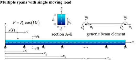
7.1 Multiple spans with single moving load ... 72

7.1.1 Formulation validation ... 72

7.1.2 Natural frequencies ... 75

7.1.3 Dynamic deflection ... 76

7.1.4 Beam with different aspect ratios ... 80

v

7.1.5 Conclusions ... 82

7.2 In thermal environment due to a moving harmonic load ... 83

7.2.1 Numerical results ... 83

7.2.2 Conclusions ... 91

7.3 Single span with multiple moving loads ... 92

7.3.1 Verification of formulation ... 93

7.3.2 Fundamental frequency ... 96

7.3.3 Effect of material non-homogeneity ... 97

7.3.4 Effect of section profile ... 99

7.3.5 Effect of distance between loads ... 101

7.3.6 Conclusions ... 103

CHAPTER 8: POST-BUCKLING ANALYSIS OF FGM STRUCTURES ... 104

8.1 Axially FGM structures ... 105

8.1.1 Rod ... 105

8.1.2 Beam and frame ... 111

CHAPTER 9: ELASTIC-PLASTIC ANALYSIS OF FGM STRUCTURES ... 117

9.1 Elastic–plastic FGM beam subjected to eccentric axial load ... 117

9.1.1 Introduction ... 117

9.1.2 Numerical examples ... 117

9.1.3 Conclusions ... 122

9.2 Elastic–plastic FGM beam on non-linear elastic foundation ... 123

9.2.1 Introduction ... 123

9.2.2 Formulation ... 124

9.2.3 Numerical results ... 125

9.2.4 Conclusions ... 137

CHAPTER 10: CONCLUDING REMARKS AND FUTURE DIRECTIONS 138 10.1 Concluding remarks ... 138

10.2 Future directions ... 139

BIBLIOGRAPHY ... 140

vi

Acknowledgements

This research was completed with much support from researchers at the Department of Architecture of the College of Engineering, Nihon University. I wish to express my sincerest gratitude to institutes and people who made substantial contributions to the completion of this dissertation as follows:

Prof. Buntara Sthenly Gan, Department of Architecture, College of Engineering, Nihon University, the supervisor of this dissertation who offered enlightened guidance, valuable comments, suggestions, assistance and encouragement towards the completion of this dissertation.

I would also like to thank my former supervisor Dr. Nguyen Dinh Kien at the Vietnam Academy of Science and Technology, Hanoi, Vietnam who played an important role providing useful comments, suggestions and guidance. And I would like to thank the members of Computational Applied Mechanics Laboratory for assisting with my stay in Japan.

I would like to thank the Ministry of Education, Culture, Sports, Science and Technology, JAPAN (MEXT Scholarship) for providing financial supports for living and tuition during my doctoral course in the College of Engineering, Nihon University.

A very special note of appreciation is expressed to my father, mother, husband and son

for their concern, self–sacrifice and encouragement both directly and indirectly for me.

1 Chapter 1: Introduction of FGM

1.1. History

Although the concept of Functionally Graded Materials (FGMs) was initiated by Japanese scientists in 1984 in Sendai [67], these sorts of materials have been exploited in numerous biological systems in nature such as bamboo, plant stems, leaf shafts or feathers, and human and animal bone, to name but a few.

(a) Bone (b) Bamboo Figure 1.1: FGM in nature

Bone and bamboo are two examples of natural FGMs displayed in Fig.1.1 as an illustration. While biological structures are living organisms that can be characterized by adaptability in order to accommodate to their physical environment, human-made FGM structures require a functional selection and combination of materials for special purposes.

1.2. FGM as new materials

FGMs have been of great importance to many researchers for a long time because

of their wide range of applications in structural mechanics. The newly-created

materials have promising applications in many fields such as space projects, the

energy sector, communications projects, the defence industries, biomedical sectors

and miscellaneous others (Figs. 1.2, 1.3). There is a comprehensive list of

2

publications on analyses of FGM structures subjected to different loadings is given in a review paper by Birman and Byrd [10]. Previously, Chakraborty [17]

employed the solutions of the governing differential equations of an FGM Timoshenko segment as interpolation functions to formulate a shear deformation beam element for analyzing the thermo-elastic behaviour of FGM beams. In 2008, Kadoli [58] formulated a beam element based on the higher-order shear deformation beam theory for studying the static behaviour of FGM beams under ambient temperature. Simultaneously, Li [75] presented a unified approach for investigating the static and dynamic behaviour of FGM beams with rotary inertia and shear deformation included. Taking the shift in position of the neutral axis into account, Kang and Li [59], [60], in the two consecutive years of 2009 and 2010, derived expressions for tip displacements of a non-linear FGM cantilever beam under a tip load or a tip moment. At the same time, Ş imş ek and his co-workers [114], [116] studied the vibration of FGM beams subjected to a moving load by using polynomial series as trial functions for the displacements and rotation of the beam. Singh and Li [119], in 2009, proposed a model for computing buckling loads of non-uniform axially FGM columns by approximating the column by another one with piecewise uniform geometric and material properties. Meanwhile, Sina [118]

presented an analytical method based on a new beam theory for free vibration analysis of FGM beams. Two years later, in 2011, Alshorbagy [1] studied the free vibration of FGM Bernoulli beams with material gradation in axial or transversal directions through the thickness by using the finite element method.

Simultaneously, Fallah and Aghdam [31] derived the non-linear governing

differential equation for geometrically non-linear vibration and post-buckling

analysis of FGM beams resting on a non-linear elastic foundation. Meanwhile,

Shahba [111] used the static solutions of a homogeneous Timoshenko beam

element to formulate the mass and stiffness matrices for computing the critical

loads and vibration characteristics of tapered Timoshenko beams made of axial

FGM. In 2014, Kocatu¨rk [68] presented the post-buckling analysis of an FGM

Timoshenko beam subjected to thermal loading by using the total Lagrangian

Timoshenko beam formulation. A year later, taking the shift in the neutral axis

position into account, Eltaher [30] derived the finite element formulation for

3

computing the natural frequencies, and showed that ignoring the shift in the neutral axis position leads to an overestimation of the computed natural frequencies. At the same year, Nguyen [91] investigated the dynamic response of functionally graded non-uniform sections of Timoshenko beams traversed by a variable speed moving load. Nguyen and his co-workers [90], [92], [93], then derived the finite element formulation for studying the large displacement behaviour of FGM beams and frames.

Figure 1.2: FGM as a new material

Figure 1.3: FGM used in ceramic–steel dental implant

4 1.3. Modelling effective FGM properties

FGMs can be formed by varying the percentage of constituents in any desired spatial direction in order to create new materials with specific physical and mechanical properties. The effective properties of the resulting material exhibit continuous change, thus eliminating the interface problem and reducing the stress concentration that is often met in conventional composites.

In general, FGMs consist of two distinct material phases of ceramic and metal alloy in order to take advantage of the good high temperature strength and creep resistance of ceramics together with the high fracture toughness and excellent thermal shock resistance of metallic materials.

Various analytical approaches to FGM modelling are reported in [56]:

• Self-consistent estimates

• Mori–Tanaka scheme

• Composite sphere assemblage model

• Composite cylindrical assemblage model

• The simplified strength of materials method

• The methods of cells

• Micromechanical model

The following three popular types of variation in constructing FGMs are reported in [56], [117]:

• The exponential law

( )

exp 1 2 z P z P

λ h

   

=   −   −     (1.1)

where

1 ln 2

t b

P λ = ^  P ^ 

  (1.2)

• The power law in the thickness direction

( ) ¹

( ) 2

n

t b b

P z P P z P

h

 

= −   +   + (1.3)

in which P(z) is the effective material properties of the FGM structure (including

5

Young’s modulus E, shear modulus G, or mass density ,...); h is the structure’s thickness; and are material properties at the top-most (z = h/2) and bottom- most (z = −h/2) surfaces, respectively; n is the non-negative power law index.

• The power law in the longitudinal direction

( )

( ) 1

n

l r r

P x P P x P

L

 

= −   −   + (1.4)

where Pl and Pr are material properties at the left-end and the right-end of the

structures, respectively; L is the total length of the structures (beam).

6 Chapter 2: Beam made of FGM

2.1 Beam theory

Beam models have been helpful in solving a large number of engineering problems.

Beam theories are extensively used to analyze the structural behaviour of slender bodies such as columns, arches, blades, aircraft wings, and bridges [33].

2.1.1 Euler–Bernoulli beam

The Euler–Bernoulli beam theory is derived from the following assumptions:

• the cross-section is rigid on its plane;

• the cross-section rotates around a neutral surface remaining in-plane;

• the cross-section remains perpendicular to the neutral surface during deformation.

Displacement field

According to the first hypothesis, the in-plane displacements u

and u

depend on the axial coordinate y only:

0 0

0

x xx

zz z

x z

xz

u x u

z

u u

z x

ε ε γ

= ∂ =

∂

= ∂ =

∂

∂ ∂

= + =

∂ ∂

(2.1)

Thus

1 1

( , , ) ( ) ( , , ) ( )

x x

z z

u x y z u y u x y z u y

=

= (2.2)

Based on the second hypothesis, axial displacement is linear versus the in-plane coordinates:

( , , )

( ) ( ) ( )

y y z x

u x y z = u y + φ y x + φ y z (2.3)

7

where and are the rotation angles along the z- and x-axis, respectively.

According to the third hypothesis and based on the definition of shear strains, the shear deformations are:

yz yx

0

γ = γ = (2.4)

The rotation angles are obtained as functions of the derivatives of displacements:

1

1

0 0

y x x

xy z

y z z

yz x

u u u

x y y

u u u

z y y

ε φ

ε φ

∂ ∂ ∂

= + = + =

∂ ∂ ∂

∂ ∂ ∂

= + = + =

∂ ∂ ∂

(2.5)

Thus

1

1 x z

z x

u y u

y φ

φ

= − ∂

∂

= − ∂

∂

(2.6)

The displacement field of the Euler–Bernoulli beam theory is then

1

1 1

1

1

x x

x z

y y

z z

u u

u u

u u x z

y y

u u

=

∂ ∂

= − −

∂ ∂

=

(2.7)

Strains

According to the kinematic hypotheses, the Euler–Bernoulli beam theory accounts for the axial strain only:

2 2

1 1 1

2 2

y y x z

yy

u u u u

x z

y y y y

ε = ^∂ = ^∂ − ^∂ − ^∂

∂ ∂ ∂ ∂ (2.8)

Stresses and stress resultants

The axial stress, , is obtained from the axial strain:

2 2

1 1 1

2 2

y x z

yy yy

u u u

E E x z

y y y

σ = ε = ^  ^∂ − ^∂ − ^{∂ } 

∂ ∂ ∂

  (2.9)

The stress resultants:

8

• axial force N(y)

  

2 2

1 1 1

2 2

2 2

1 1 1

2 2

( )

x z

yy

y x z

y x z

A S S

N y d

u u u

E x z d

y y y

u u u

E d xd zd

y y y

σ

Ω

Ω

Ω Ω Ω

= Ω

∂

 ∂ ∂ 

=  − −  Ω

∂ ∂ ∂

 

 

 ∂ ∂ ∂ 

=  Ω − Ω − Ω 

∂ ∂ ∂

 

 

 





  

(2.10)

• bending moment versus the z-axis Mz (y)



2 2

1 1 1

2 2

2 2

1 1 2 1

2 2

( )

x xx xz

z yy

y x z

y x z

S I I

M y xd

u u u

E x z xd

y y y

u u u

E xd x d xzd

y y y

σ

Ω

Ω

Ω Ω Ω

= Ω

∂

 ∂ ∂ 

=   ∂ − ∂ − ∂   Ω

 

 ∂ ∂ ∂ 

 

= Ω − Ω − Ω

∂ ∂ ∂

 

 

 





  

 

(2.11)

• bending moment versus the x-axis M

(y)



2 2

1 1 1

2 2

2 2

1 1 1 2

2 2

( )

z xz xx

x yy

y x z

y x z

S I I

M y zd

u u u

E x z zd

y y y

u u u

E zd xzd z d

y y y

σ

Ω

Ω

Ω Ω Ω

= − Ω

∂

 ∂ ∂ 

= −   ∂ − ∂ − ∂   Ω

 

 ∂ ∂ ∂ 

 

= − Ω − Ω − Ω

∂ ∂ ∂

 

 

 





  

 

(2.12)

where A is the cross-section area; S

and S

are static momenta; and I

, I

and I

are momenta of inertia. Eqs. (2.10), (2.11) and (2.12) can be written in matrix form:

1 2 3

x z

z x zz xz

x z xz xx

A S S k

N

M S I I k

M S I I k

 

   

  =    

     

 −     

     

(2.13)

9 2.1.2 Timoshenko beam

In the Timoshenko beam theory, the third kinematic a priori assumption of the Euler–

Bernoulli beam theory is relaxed.

Displacement field

According to the previous a priori kinematic assumptions, the displacement field of the Timoshenko beam theory is

1 1 1

( , , ) ( )

( , , ) ( ) ( ) ( ) ( , , ) ( )

x x

y y z x

z z

u x y z u y

u x y z u y y x y z u x y z u y

φ φ

=

= + +

=

(2.14)

Strains

1

1

1

y y z x

yy

y x x

xy z

y z z

yz x

u u

x z

y y y y

u u u

x y y

u u u

z y y

φ ε φ

γ φ

γ φ

∂ ∂ ∂ ∂

= = + +

∂ ∂ ∂ ∂

∂ ∂ ∂

= + = +

∂ ∂ ∂

∂ ∂ ∂

= + = +

∂ ∂ ∂

(2.15)

Stresses and stress resultants

1

1

1

y z x

yy yy

xy z x

yz x z

E E u x z

y y y

G u

y G u

y

φ σ ε φ

σ κ φ

σ κ φ

∂

 ∂ ∂ 

= =   ∂ + ∂ + ∂  

 ∂ 

=   + ∂  

 ∂ 

=   + ∂  

(2.16)

where κ is the shear correction factor.

The stress resultants

• axial force N(y)

1 yy

y z x

N d

E u x z d

y y y

σ

φ φ

Ω

Ω

= Ω

∂

 ∂ ∂ 

=   ∂ + ∂ + ∂   Ω



 ^(2.17)

10

• bending moment versus the z-axis M

1 2

z yy

y z x

M zd

E u z xz z d

y y y

σ

φ φ

Ω

Ω

= Ω

∂

 ∂ ∂ 

=   ∂ + ∂ + ∂   Ω



 ^(2.18)

• bending moment versus the x-axis M

1 2

x yy

y z x

M xd

E u x x xz d

y y y

σ

φ φ

Ω

Ω

= − Ω

∂

 ∂ ∂ 

= −   ∂ + ∂ + ∂   Ω



 ^(2.19)

• shear force along the x-axis V

1

1

x xy

z x

z x

V d

G u d

y

G u A

y σ

κ φ κ φ

Ω

Ω

= Ω

 ∂ 

=   + ∂   Ω

 ∂ 

=   + ∂  



 (2.20)

• shear force along the z-axis V

1

1

z yz

z x

x z

V d

G u d

y

G u A

y σ

κ φ κ φ

Ω

Ω

= Ω

 ∂ 

=   + ∂   Ω

 ∂ 

=   + ∂  



 ^(2.21)

11 2.2. FGM in beam theory

2.2.1. Prismatic FGM beam

Consider the beam to have a cross-section assumed to be rectangular with width b and height h (Fig. 2.1).

x z

section A-B A

B

z

b

h h

generic beam element u

w

θ

^u

w

θ

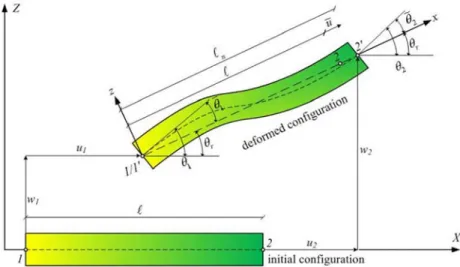
Figure 2.1: FGM beam and its generic element

The beam material is assumed to be an FGM composed of two constituent materials, and the effective material properties are graded in the thickness direction (z-direction) according to a power law distribution as

( )

( ) ( ) 1

2 1

n

b t b

n t

t b

P z P P P z h V z z

h V V

= + −    

 

 

=   +   + =

(2.22)

where P(z) represents the effective material properties, including Young’s modulus,

shear modulus and mass density; P

and P

are the material properties of the

material at the top and bottom surfaces, respectively. and respectively denote

the volume fractions of the materials at the top and bottom surfaces; n is the non-

negative power-law index, which defines the distribution of the constituent

materials.

12

Figure 2.2: Variation in volume fraction through the thickness of FGM beams Fig. 2.2 shows the variation in the volume fraction through the beam thickness for various values of the index n of the FGM beam. Due to variation of the effective Young’s modulus, the neutral axis is no longer at the mid-plane, but it shifts from the mid-plane by a distance h

, which can be determined by imposing the axial resultant in a cross-section that vanishes:

x

0

A

N =  σ dA = ^(2.23)

then

( )

( )( )

/2

/2

0 /2

/2

( )

2 2

( )

h

t b

h h

t b

h

E z zdz

hn E E

h n E nE

E z dz

−

−

= = −

+ +



 ^(2.24)

Adopting Timoshenko beam theory, the axial and transverse displacements, u

(x, z, t) and u

(x, z, t), respectively at any point of the beam are given by

1 3

( , , ) ( , ) ( , ) ( , , ) ( , )

u x z t u x t z x t u x z t w x t

θ

= −

= (2.25)

where u(x,t) and w(x, t) are the axial and transverse displacements of the point on

the neutral axis x; θ(x, t) is the rotation of the cross-section at a point with abscissa

13

x; z is the distance from any arbitrary point to the neutral axis.

Based on the assumptions of Hooke’s law, the axial strain ε

, shear strain γ

and their corresponding axial and shear stresses, σ

and τ

, respectively, are as follows:

( , ) ( , ) ( , )

( , ) ( )

( )

x

xz

x x

xz xz

u x t x t

x z x

w x t x x t E z

G z ε θ

γ θ

σ ε

τ κ γ

∂ ∂

= −

∂ ∂

= ∂ −

∂

=

=

(2.26)

The strain energy of the beam can be written as

( )

2 2 2

11 12 22 33

0

1 2

1 2

2

x x xz xz

V l

U dV

u u w

A A A A dx

x x x x x

σ ε τ γ

θ θ κ θ

= +

  ∂  ∂ ∂  ∂   ∂  

=      ∂   − ∂ ∂ +   ∂   +   ∂ −     





(2.27)

Kinetic energy is written as

( )

( )

2 2

2 2 2

11 12 22

0

1 ( ) 2

1 2

2

V l

T z u w dV

I u w I u I dx

ρ

θ θ

= +

 

=  + − + 





 

 

  

(2.28)

where κ is the shear correction factor; E(z), G(z) and ρ(z) are the Young’s modulus, shear modulus and mass density of the material on the section with abscissa z; V is the volume; an over dot symbol denotes the time derivative; the stiffness coefficients and mass moment of inertia in Eq. (2.27) are defined as

( ) ( )

( ) ( )

2

11 12 22

33

2 11 12 22

, , ( ) 1, ,

( )

, , ( ) 1, ,

A

A

A

A A A E z z z dA

A G z dA

I I I ρ z z z dA

=

=

=







(2.29)

where A is the cross-section area.

It should be noted that due to the shift in the neutral axis position, the integrals in Eq.

(2.29) should be computed in the manner described by Kang and Li [59], [60].

14

0 0

0 0

0 0

11 0 0

0 0

12 0 0

0 0

2 2 2

22 0 0

0 0

33 0

( ) ( ) ( ) ( )

( ) ( ) ( ) ( )

( ) ( ) ( ) ( )

( ) ( ) ( ) (

h h h

A

h h h

A

h h h

A

A

A E z dA b x E h z dz E h z dz A zE z dA b x zE h z dz zE h z dz A z E z dA b x z E h z dz z E h z dz

A G z dA b x G h z dz G

−

−

−

 

= =  + + − 

 

 

 

= =  + + − 

 

 

 

= =  + + − 

 

 

= = + +

  

  

  



0 0

0 0

0 0

0

0 0

11 0 0

0 0

12 0 0

0 0

2 2 2

22 0 0

0 0

)

( ) ( ) ( ) ( )

( ) ( ) ( ) ( )

( ) ( ) ( ) ( )

h h h

h h h

A

h h h

A

h h h

A

h z dz

I z dA b x h z dz h z dz

I z z dA b x z h z dz z h z dz

I z z dA b x z h z dz z h z dz

ρ ρ ρ

ρ ρ ρ

ρ ρ ρ

−

−

−

−

 

−

 

 

 

 

= =  + + − 

 

 

 

= =  + + − 

 

 

 

= =  + + − 

 

 

 

  

  

  

(2.30)

2.2.2. FGM beam in thermal environment

The beam with total length L, cross-section height h and cross-section width b, shown in Fig. 2.3, will be investigated in this sub-section.

Figure 2.3: A simply supported FGM beam in thermal environment

The x-axis is chosen to be on the mid-plane, and the z-axis is perpendicular to the mid-plane. The beam material is formed from ceramic and metal, where the volume fraction of ceramic ( Vc ) and metal ( Vm ) is assumed to be given by

1 2 1

n c

m c

V z h

V V

 

=   +   + =

(2.31)

15 where n (0 ≤ n < ∞) is the grading index.

In Eq. (2.31), the subscripts “c” and “m” are used to indicate ceramic and metal, respectively. The beam material is considered to be dependent on the temperature, and a typical property (P) is a function of temperature (T) as [132]

(

)

0 1

1

P P P T =

+ + PT PT + + PT (2.32) where T=T

+∆T, in which T

= 300K is the reference temperature and ∆T is the temperature rise, in the current environment temperature; P

, P

, P

, P

and P

are coefficients of T and they are unique to the constituents. The effective material properties are evaluated by Voigt’s model:

( , )

( )

( )

P z T = P T V + P T V (2.33)

From Eqs. (2.31) and (2.33), the effective Young’s modulus, thermal expansion and mass density are given by

[ ]

[ ]

( , ) ( ) ( ) 1 ( )

2

( , ) ( ) ( ) 1 ( )

2 ( ) ( ) 1

2

n

c m m

n

c m m

n

c m m

E z T E T E T z E T

h

z T T T z T

h z z

h

α α α α

ρ ρ ρ ρ

 

= −   +   +

 

= −   +   +

 

= − +   +   +

(2.34)

where the mass density is considered to be independent of the temperature. In this work, the temperature is considered to vary in the thickness direction only, and it is assumed that the temperature being imposed is Tm at the bottom surface and Tc at the top surface. With this condition, the distribution of temperature in the thickness can be obtained as the solution of the following Fourier equation:

( ) 0

d dT

dz K z dz

 

−     = (2.35)

where K(z) is the thermal conductivity, assumed to be independent of the

temperature. The solution of Eq. (2.35) has the form

16

/2

/2 /2

( ) 1

( , ) 1

( , )

z

c m

c h

h h

T T

T T dz

K z T K z T dz

−

−

= + − 

 ^(2.36)

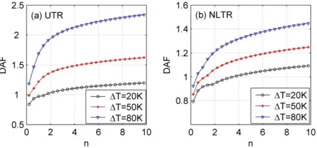
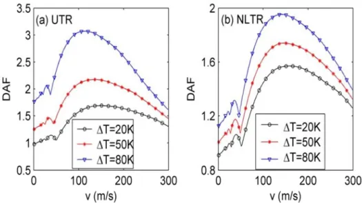
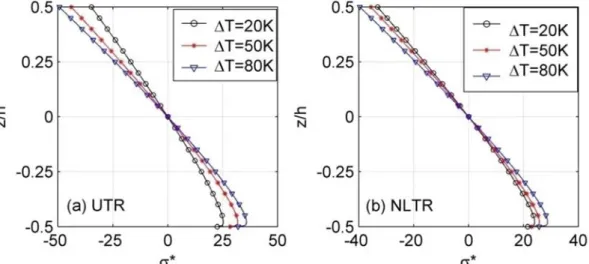
If T

=T

, Eq. (2.36) gives a uniform temperature rise (UTR). Otherwise, it describes a non-linear temperature rise (NLTR).

2.2.3. Non-prismatic FGM beam

The beam shown in Fig. 2.4, with total length L and a constant cross-section height h, is assumed to be formed from two different materials.

Figure 2.4: Two types of non-prismatic FGM beam

The solid cross-section area A(x) and moment of inertia I(x) are assumed to vary longitudinally in the two following manners:

• Type A

( ) 1 1

2 ( ) 1 1

2

m

m

A x A x

L I x I x

L α α

 

=  − − 

 

 

=  − − 

 

• Type B

2

2

( ) 1 1

2 ( ) 1 1

2

m

m

A x A x

L I x I x

L α α

 

=  − − 

 

 

=  − − 

 

where A

, and I

denote the area and moment of inertia of the mid-span section,

17

respectively. 0 ≤ < α 2 is the non-uniform section parameter, defining how the cross- section varies. The effective property P (Young’s modulus, shear modulus and mass density) of the beam is assumed to vary in the longitudinal direction according to a power law equation as

( ) ( ) 1

n

l r r

P x P P x P

L

 

= −  −  +

  (2.37)

where n is a non-negative power law index, which defines the distribution of the constituents along the longitudinal direction of the beam. The lower subscripts “l” and

“r” stand for “left” and “right”, respectively. As seen from Eq. (2.37), the left and right end sections of the beam contain one pure material. Adopting Timoshenko beam theory, the axial and transverse displacements, u

(x, z, t) and u

(x, z, t), respectively at any point of the beam are given by

1

3

( , , ) ( , ) ( , ) ( , , ) ( , )

u x z t u x t z x t u x z t w x t

θ

= −

= (2.38)

where u(x, t) and w(x, t) are the axial and transverse displacements of the point on the neutral axis x; θ(x, t) is the rotation of the cross-section at a point with abscissa x; z is the distance from any arbitrary point to the neutral axis. Based on the assumptions of Hooke’s law, the axial strain ε

, shear strain γ

and their corresponding axial and shear stresses, σ

and τ

, respectively, are as follows:

( , ) ( , ) ( , )

( , ) ( )

( )

x

xz

x x

xz xz

u x t x t

x z x

w x t x x t E x

G x ε θ

γ θ

σ ε

τ κ γ

∂ ∂

= −

∂ ∂

= ∂ −

∂

=

=

(2.39)

The strain energy and the kinetic energy for the non-uniform FGM Timoshenko beam

can be written in the following forms:

18

2 2

0 2

2 2 2

0

( ) ( ) ( ) ( ) 1

2 ( ) ( )

1 ( ) ( )( ) ( ) ( ) 2

l

l

E x A x u E x I x

x x

U dx

G x A x w x

T x A x u w x I x

θ

κ θ

ρ ρ θ

  ∂  +  ∂  + 

   ∂     ∂   

 

=        ∂ ∂ −       

 

=  + + 



 ^{  }

(2.40)

where E(x), G(x), ρ(x) are the Young’s modulus, shear modulus and mass density of the material on the section with abscissa x.

2.2.4. Elastic–plastic FGM beam

Figure 2.5 shows a cantilever FGM beam made of ceramic and metal.

Figure 2.5: A cantilever FGM beam made of ceramic and metal

L, h, b denote the length, height and width of the beam, respectively. The volume fractions of the two constituent materials follow a simple power-law function:

1 2 1

n c

c m

V z h V V

 

=   +   + =

(2.41)

where z is the transverse coordinate; V

and V

are respectively the volume

fractions of ceramic and metal, and n is the volume fraction exponent; the

subscripts “c” and “m” stand for “ceramic” and “metal”, respectively. The linear

elastic behaviour of FG material is described by Hooke’s law, and its effective

material properties can be evaluated by micromechanics models used in

conventional composites. The elastic–plastic behaviour of ceramic/metal FG

materials is widely described by using the Tamura–Tomota–Ozawa (TTO) model

19

[121]. According to this model, the uniaxial stress σ and strain E of a two-phase composite are related to the corresponding average uniaxial stresses and strains of the two constituent materials [42], [55]:

c c m m

c c m m

V V

V V

σ σ σ

ε ε ε

= +

= + (2.42)

In the TTO model, an additional parameter q representing the ratio of stress to strain transfer is introduced as

, 0 q

c m

c m

q σ σ

ε ε ^<

−

= − < ∞ (2.43)

The value of q depends on the properties of the constituent materials and the micro- structural interaction in the composite.

In the TTO model for a ceramic/metal FGM, the ceramic phase is assumed to be linearly elastic during its deformation process. Plastic deformation of the composite arises from plastic flow of the metal phase when the stress exceeds its yield limit.

Here, a bilinear stress–strain relation with an isotropic hardening is assumed for the elastic–plastic behaviour of metal. Figure 2.6 represents a constant tangent modulus E

when the stress in the metal phase exceeds its yield limit σ

.

The elastic–plastic behaviour of the ceramic/metal FGMs also follows a bilinear isotropic hardening model representing a tangent modulus Et in the plastic region (blue lines in Fig. 2.6).

Figure 2.6: Bilinear elastic-plastic model for FGM

The effective properties such as Young’s modulus E, yield stress and tangent

modulus E

of the FGM are evaluated from the corresponding parameters of

constituent materials and the parameter q by using the TTO model as

20

( ) ( )

( )

0

c m m c c

m

c m c

m

m c c

Y Ym m c

c m m

c

m c c

t

c m c

m

q E E V E V E z q E

q E V V q E

q E E E

z V V

q E E E q E E V E V E z q E

q E V V q E

σ σ

 + + 

 + 

 

=    + + +   

 + 

=   + +  

 + + 

 + 

 

=    + + +   

(2.44)

where E(z) is the elastic modulus; σ

(z) is the yield stress, and E

(z) is the tangent modulus; E

, E

are the Young’s modulus of the ceramic and metal constituents, respectively; E

, σ

are the tangent modulus and yield stress of the metal constituent; and the parameter q is the ratio of stress to strain transfer between the two constituents.

Since the Young’s modulus of the composite varies asymmetrically, the neutral axis of the beam is no longer on the mid-plane, but it shifts from the mid-plane by a distance h

, which can be determined by imposing the axial resultant in a cross- section that vanishes:

/2

/2

0 /2

/2

( ) 0

( )

h

h

x h

A

h

E z zdz

N dA h

E z dz

σ

−

= =  = 

  ^(2.45)

In order to calculate h

, Simpson’s rule is employed for numerical integration. The rule is described as follows:

( ) ( ) 4 ( )

6 2

b

a

b a a b

f x dx ≈ −    f a + f    +    + f b   

 ^(2.46)

Adopting the neutral surface as the reference plane, the axial and transverse

displacements at any point according to Euler–Bernoulli beam theory are as

follows:

21

1 0

2

3

( )

0 ( ) u u z h w

x u

u w x

= − − ∂

∂

=

=

(2.47)

where u

, u

and u

are the displacements at any point in directions of the x-, y- and z-axes. A degenerated form of Green strain can be adopted for the elastic–plastic analysis as

0 0 0

1 ( ) ( )

2

u w

z h z h

x x

ε = ^∂ + ^∂ + − χ ε = + − χ

∂ ∂ (2.48)

where

¹

2

u w

x x

ε = ^∂ + ^∂

∂ ∂ is the membrane strain, and

2 2

w χ = − ^∂ x

∂ is the beam curvature.

The incremental stress–strain relationship for the one-dimensional elastic–plastic analysis can be written in the form

d σ = E d

ε (2.49)

where E

is the instantaneous modulus, and for the bilinear model adopted herein it has followed the simple form

Y ep

t Y

d E if

E d E if

σ σ σ

σ σ ε

≤

= =  

 > (2.50)

where and E

are the yield stress and tangent modulus of the FGM, respectively.

22 2.3. Shape functions

2.3.1. Classical formulation

In the classical formulation for shape functions, linear functions N

^{L x} L

= − and

2 u

N x

= L are used to interpolate the axial displacement u while the Hermite polynomials are applied for interpolation of transverse displacement w and rotation θ. Steps to build the Hermite shape functions are as follows:

Nodal vector { } { ^{q = w}

^θ

^w

^θ

}

Length L of the beam is scaled to 1 using scaling parameter s:

1

1 s x x

L ds dx

L

= −

=

(2.51)

The deflection curve w(s) in terms of s by using cubic functions can be written as

2 3

0 1 2 3

( )

w s = + a a s a s + + a s (2.52) The rotation

(

)

1 2 3

dw dw ds

a a s a s dx ds dx L

θ = = = + + (2.53)

Applying boundary conditions

1 2

1 2

(0) , ( )

(0) , ( )

w w w L w

dw dw

dx θ dx L θ

= =

= = (2.54)

we have

23

( )

1 0

1 1

1 0 1 2 3

1 1 2 3

(0) (0) 1

( )

( ) 1 2 3

w w a

dw a

dx L

w w L a a a a

dw L a a a

dx L

θ

θ

= =

= =

= = + + +

= = + +

(2.55)

Expressing four coefficients (a

, i=0..3) in nodal terms, one can obtain

0 1

1 1

2 1 1 2 2

3 1 1 2 2

3 2 3

2 2

a w

a L

a w L w L

a w L w L

θ

θ θ

θ θ

=

=

= − − + −

= + − +

(2.56)

Replacing back into w(s)

2 3 2 3

1 1

2 3 2 3

2 2

( ) (1 3 2 ) ( 2 )

(3 2 ) ( )

w s s s w L s s s

s s w L s s

θ θ

= − + + − +

+ − + − + (2.57)

or one can rewrite

[ ]

1 1

1 2 3 4

2 2

( ) ( ) ( ) ( ) ( )

w

w s N s N s N s N s

w θ θ

   

=    

   

 

(2.58)

where N

(s), (i=1..4) are called Hermite shape functions:

2 3

1

2 3

2

2 3

3

2 3

4

( ) 1 3 2

( ) ( 2 )

( ) 3 2

( ) ( )

N s s s

N s L s s s

N s s s

N s L s s

= − +

= − +

= −

= − +

(2.59)