Abstract
This paper estimates the one-day-ahead Value-at-Risk (VaR) and the one-day- ahead expected shortfall (ES) of daily returns for the Standard&Poorʼs 500 (S&P500) stock index. The predictive ability of the VaR forecasts and the ES forecasts are evaluated via the associate backtesting methods. Return volatil- ity defined as the standard deviation or variance of daily return, which is essential to the calculation of VaR and ES, is estimated by applying the observations to the stochastic volatility (SV) model and the realized stochas- tic volatility (RSV) model.
Although many empirical studies show that with the introduction of high frequency intraday returns data, the RSV model performs better over the basic SV model, the difference in time spans should also be taken into consid- eration. To investigate the sensitivity to the choice of the time span of observations, this paper estimates the volatilities of a relatively long time period from the years 2000 to 2016, along with two short periods before and after the financial crisis of the year 2008 separately. Empirical evidence dem- onstrates that volatility forecasts generated from the RSV model outperform those from the SV model for the short time periods of the years 2000-2007 and 2009-2016, while the conclusion for the long time period of years 2000- 2016 is the opposite. Therefore, with respect to the S&P500 stock index, the RSV model fits the data of shorter time spans better, while the SV is more capable for the data of longer time span.
An Empirical Study of Quantile Forecasts for the S&P500 Stock Index
Chao LU
早稲田商学第451・452合併号
2 0 1 8 年 3 月
1. Introduction
The risk measure of VaR is typically used as quantile forecast of financial returns in financial risk management. To obtain the VaR forecast, it is also required to predict the unobservable variable of volatility. In practice, para- metric approaches such as autoregressive conditional heteroskedasticity (ARCH) models and SV models, and nonparametric estimators such as real- ized volatility (RV) and realized kernel (RK) are commonly applied to estimate the volatility.
The parametric approaches aim to establish certain models to describe the dynamics of the latent volatility. The ARCH-type models, including the under- lying ARCH model proposed by Engle (1982), the GARCH (generalized ARCH) model proposed by Bollerslev (1986) and a variety of other extension models, consider volatility at date to be a deterministic function of the known variable at date -1. This assumption, however, is not in keeping with the situations of real markets. Alternatively, this paper applies the returns data to the SV model developed by Taylor (1986) where volatility is taken as an unknown parameter. It is notable that only the financial daily returns data are used either in an ARCH model or in a SV model, and thus some intraday information may be lost for such models.
On the other hand, nonparametric methods acquire the estimate of latent volatility based on the high frequency intraday returns data, among which RV proposed by Andersen and Bollerslev (1998) and Barndorff-Nielsen and Shephard (2001) is widely used. This realized measure, however, usually turns out to be an inconsistent estimator of the latent volatility due to the influence of non-trading hours and market microstructure noise (MMN) that appear in real markets.
Takahashi, Omori, and Watanabe (2009) propose to model daily returns and RVs simultaneously to a RSV framework to account for the information loss of daily returns and the bias of RV caused by non-trading hours and MMN.
This paper also estimates this RSV model to explore the model fitting.
The VaR can be computed easily given the volatility forecast and the returns distribution. However, VaR only focuses on the quantile and thus it is insensitive to the shape of the tail of the returns distribution. To cope with this problem, ES is also estimated to capture the further information of tail distribution. These VaR and ES forecasts are evaluated with their corre- sponding backtesting procedures, in addition to computing several loss functions on predictive performance of the volatility forecasts.
This paper is organized as follows. Section 2 briefly introduces the SV and RSV models for volatility forecasts and the risk measures for quantile fore- casts. Section 3 illustrates the estimation approaches and the evaluation methods for the one-day-ahead VaR and ES forecasts. Empirical results are analyzed in Section 4. Conclusions are given in section 5.
2. Models and Quantile Forecasts
Return volatility of date is defined as the integral of the instantaneous vola- tility s2( ) over the interval of ( , +1):
(1)
The SV model specified as follows is established as a parametric method to estimate latent variable in equation (1):
(2)
(3)
where denotes the daily return and denotes the logarithm of latent vola- tility. Suppose that ( - m) follows a stationary AR(1) process with |f |<1 and the initial value 1 follows a Gaussian distribution with an unconditional mean
1 2( ) .
t
t t
IV =
∫
+s s dsexp( / 2) ,
t t t
R = h e
1 ( ) ,
t t t
h+ =m f+ h -m η+
η
η η
e rs
η rs s
=
2
( , ), 1 .
t t
N 0Σ Σ
and variance of , that is, 1~ (m,sη2/(1-f2)). This paper also assumes that e and η follow a bivariate normal distribution. r, which represents the correla- tion coefficient of and +1, can explain the asymmetric phenomenon and is usually evaluated to be negative mainly due to the leverage effect and the volatility feedback effect.
On the other hand, RV defined as the sum of squared intraday returns over day , is also widely used as a nonparametric estimator of latent volatil- ity.
(4)
where { ,}=0-1 represents the intraday returns data of date . As stated in Section 1, this nonparametric estimator is usually inconsistent with latent vol- atility in real markets where non-trading hours and MMN exist.
Takahashi, Omori and Watanabe (2009) develop the following RSV model to incorporate the SV model with the RV:
(5)
(6)
(7)
where denotes the logarithm of realized volatility of date . Equations (5) and (6) are the basic SV model. The sign of ξ in equation (7) shows the domi- nant effect of MMN and non-trading hours. A positive estimate of ξ indicates an upward bias due to MMN, while a negative ξ suggests a downward bias due to non-trading hours.
Let θ denote the parameter vector (m, f, r, sη2, ξ, s2)′ and h denote the vol-
1 2 , 0
,
n
t t i
i
RV r
-
=
=
∑
exp( / 2) ,
t t t
R = h e
1 ( ) ,
t t t
h+ =m f+ h -m η+
t t t,
x = +ξ h +u
η
η η
e rs
η rs s
s
=
2
2
1 0
( , ), 0 .
0 0
t t
t u
N u
0Σ Σ
atility vector ( 1, 2, …, )′. Given the observations R=( 1, 2, …, )′ and X=( 1, 2, …, )′, where is the sample size of the observations, samples of θ and h can be drawn recursively from the joint conditional posterior density
via MCMC-based Bayesian method.
Based on the estimation results, the one-day-ahead VaR forecast of date +1 given the information up to date (I) with probability a is defined as
(8)
In spite of its extensive utilization in the area of financial risk management, VaR is a yet imperfect measure for the reason that it simply discusses the quantile of the returns distribution and overlooks the information of the tail distribution. This problem is settled by developing another measure referred to as ES to account for the returns distribution that is beyond the quantile.
The one-day-ahead ES forecast of +1 with probability a is given by
(9)
3. Estimation and Evaluation
This section interprets the computational algorithms and evaluation methods for one-day-ahead VaR and ES forecasts. Additionally, two loss functions are also introduced to evaluate the predictive ability of the volatilities to make comparisons between the two SV models.
3.1 Estimation of the VaR and ES forecasts
By applying the previous 0 observations to the RSV model recursively, the one-day-ahead VaR forecasts { a 0+}=1 and one-day-ahead ES forecasts { 0+}=1can be calculated according to the following algorithm, where
= - 0 represents the number of VaR or ES forecasts.
Step 1. Set =1.
Step 2. Generate θ =(m, f, r, sη2, ξ, s 2)′ and h=( 1, 2, …, 0)′ from the
1 1
( t t ( ) t) .
Pr R+ <VaR+ a I =a
1( ) 1 1 1( ), .
t t t t t
ES+ a =E R + R+ <VaR+ a I
joint conditional posterior density p(θ,h R,X).
Step 3. Generate the sample of logarithm of one-day-ahead volatility from the posterior predictive distribution:
where the conditional mean and variance are given by
Step 4. Compute a 0+ (a)=exp( 0+1/2) (a), where (a) is the a-quantile of returns distribution.
Step 5. Randomly generate samples of from the returns distribution, where is set to be a sufficiently large enough number, and com- pute the corresponding { 0+} =1 using 0+ =exp( 0+1/2) .
Step 6. Calculate 0+ (a) = [ 0+ | 0+ < a 0+i(a), I 0+ -1], which is the average of the violated 0+.
Step 7. Set = +1, repeat from Step 2 if < and end if = .
The Bayesian based MCMC method is used to generate the RSV model in Step 2 on account that the nonlinear specified measurement equation (5) will make it difficult to carry out the maximum likelihood estimation (MLE). The details of generation algorithm for RSV model are described in appendix A.
This algorithm is also available for SV model simply by substituting the parameter vector (m, f, r, sη2, ξ, s2)′ to (m, f, r, sη2)′.
3.2 Evaluation of the VaR and ES forecasts
This subsection explains the principles of several backtesting methods used to investigate the robustness of the predicted VaR and ES estimates.
Suppose that the number of the violated VaR forecasts among { 0+ (a)}=1 is . Then the empirical failure rate (EFR) can be written as = / . This paper tests the null hypothesis of =a by calculating the following likelihood ratio (LR) statistic (Kupiec (1995)):
(10)
2
0 1 ( 0 1, 0 1),
i i i
T T T
h + ⋅N m + s +
2 2 2
0 1 ( 0 ) exp( 0/ 2), 0 1 (1 ).
i i i i i i i i i i i
T hT ηRt hT T η
m + =m +f -m +r s - s + =s -r
{ }
2 log Tv(1 )Tf Tv log Tv(1 )Tf Tv . LR= EFR -EFR - - a -a -
This statistic is asymptotically distributed as a χ2(1) under the condition that the null hypothesis is true.
The measure (a) proposed by Embrechts, Kaufmann, and Patie (2005) is computed to backtest the ES forecasts. Specifically, define δ (a)= - (a) and denote (a) as the empirical a-quantile of δ(a). Let k1(a) and k2(a) be the sets of time points for which δ(a)<0 occurs and δ(a)< (a) occurs, respec- tively. Suppose that the respective number of k1(a) and k2(a) are counted to be 1 and 2, then the measure is written as
(11)
where
(12)
This measure considers to average the absolute values of the standard back- testing measure 1(a) and the penalty term 2(a). A lower value of (a) indicates better ES forecasts.
Moreover, two loss functions, which are the mean squared error (MSE) and the quasi-likelihood (QLIKE), defined as equations (13) and (14), respectively, are calculated to measure the precision of the volatility forecasts, of which values can provide further information about the predictive performance.
(13)
(14)
where s^2+1| and s2+1 denote one-day-ahead volatility forecast and volatility proxy of date +1. As stated in Patton (2011), these two loss functions can lead to [s^2t+1| |I]=s2+1, which is a necessary condition for a loss function to be robust to noise in the volatility proxy.
This paper uses the scaled realized kernel (SRK) proposed by Hansen and Lunde (2005) as the proxy of latent volatility. The SRK is specified as the
(
1 2)
( ) 1 ( ) ,
2 ( )
Da = D a + D a
1 2
1 2
1 ( ) 2 ( )
1 1
( ) t( ), ( ) t( ).
t t
D D
T k a T k a
a δ a a δ a
∈ ∈
=
∑
=∑
( )
0
1 2
2 2
1 1
1 ,
T
t t t f t T
MSE T − σ+ σ +
=
=
∑
ˆ −0
2
1 2
2 1
1 2
1
1 ,
T
t t t
f t T t t
QLIKE log
T
σ σ σ
− + +
= +
= +
∑
ˆ ˆproduct of the RK and the ratio of the variance of daily return to the mean of RKs. This specification makes it possible to adjust the underestimation caused by non-trading hours.
(15)
MMN, which is the primary reason that causes significant increase of bias in RV when the time interval is close to zero, is accounted by the estimator of RK proposed by Barndorff-Nielsen, Hansen, Lunde, and Shephard (2008).
(16)
where H is the bandwidth of autocovariance lag, gh represents the autocovari- ance at lag with high frequency data { }:
(17)
and weight ( ) represents the Parzen kernel function defined as:
(18)
4. Empirical Results
In this section, daily returns and 5-minute RVs of S&P500, provided by the Oxford-Man Instituteʼs Realized Library, are applied for empirical estimation.
The sample period is from January 4, 2000 to December 30, 2016, and the sample size is 4247.
In order to investigate the model fitting with respect to different time spans, this paper also estimates the volatilities of the years 2000-2007 and 2009-2016, respectively. The year 2008 is excluded to avoid the contaminated time period of financial crisis. The computational results were generated by using the MATLAB̲R2015b software.
2 1
1
( )
, .
T t t
t t T
t t
R R SRK cRK c
RK
=
=
= =
∑
-∑
1 .
H
t h
h H
RK k h
H g
=-
=
∑
+ 1
,
n
h j j h
j h
g r r-
= +
=
∑
( )
2 3
3
1 6 6 , 0 1 / 2
( ) 2 1 , 1 / 2 1.
0, 1
x x x
k x x x
x
- + ≤ ≤
= - ≤ ≤
>
4.1 Descriptive Statistics
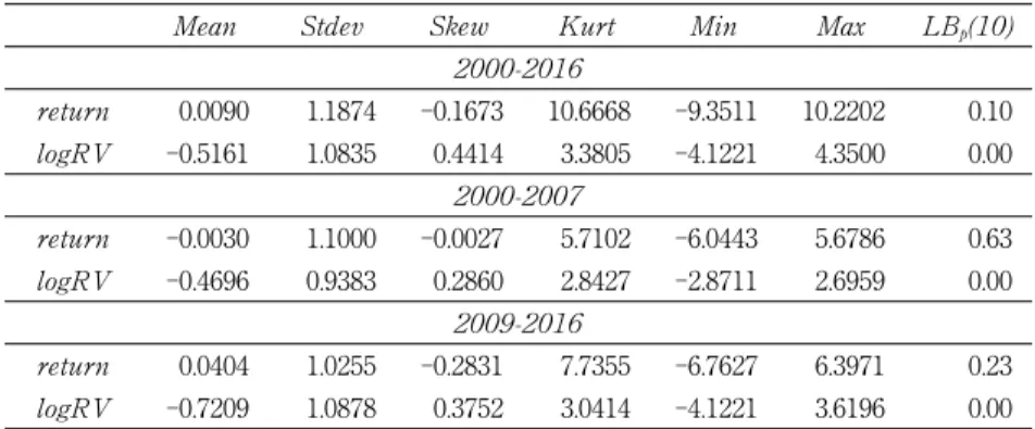
Table 1 shows the descriptive statistics of daily returns (in percentage) and the logarithm of RVs for the respective time spans. ( ) represents the -value of the Ljung-Box (LB) statistics, whose null hypothesis is no autocor- relation up to lags. Following Diebold (1988), the ( ) statistics of returns and logRVs modified for heteroscedasticity are described as
(19)
(20)
where s^4 and s^4 are the squared sample variance of daily returns and logRVs, g 2( ) and g 2( ) are the -th order autocovariance of sequence {( - )2}=1 and {(log -log )2}=1, r^2( ) and r^2 ( ) are the squares of -th order auto- covariance of returns and logRVs. The statistic is asymptotic to a χ2( ) distribution on the condition that the null hypothesis is true.
2
4 2
4 1
( ) ( 2) ( ),
( )
m
R R
return
k R R
LB m T T k
T k k
σ ρ
σ γ
=
= +
∑
ˆ +ˆ ˆ −2
4 2
4 1
( ) ( 2) ( ),
( )
m
RV RV
RV
RV
k RV
LB m T T k
T k k
σ ρ
σ γ
=
= +
∑
ˆ +ˆ ˆ −Table 1. Descriptive Statistics
0.0090 1.1874 ‑0.1673 10.6668 ‑9.3511 10.2202 0.10
‑0.5161 1.0835 0.4414 3.3805 ‑4.1221 4.3500 0.00
‑0.0030 1.1000 ‑0.0027 5.7102 ‑6.0443 5.6786 0.63
‑0.4696 0.9383 0.2860 2.8427 ‑2.8711 2.6959 0.00
0.0404 1.0255 ‑0.2831 7.7355 ‑6.7627 6.3971 0.23
‑0.7209 1.0878 0.3752 3.0414 ‑4.1221 3.6196 0.00
NOTE: The sample periods are 2000-2016, 2000-2007 and 2009-2016 where the respective sample sizes are 4247, 1987 and 2014. (10) shows the value of the Ljung-Box statistic up to 10 lags for the returns and realized measures where the heteroskedasticity is corrected following Diebold (1988).
The means of daily returns are not statistically significant from zero, and the (10) statistics do not reject the null hypothesis of no autocorrelation at the 10% significance level. As a result, there is no need to adjust the means and autocorrelations of the daily returns. In contrast, the null hypothesis that no autocorrelation extists at the 1% significance level are rejected for the cases of logRV, which indicate the high serial correlation of logarithm of volatilities.
4.2 Estimation Results
Tables 2-3 describe the posterior means, the standard deviations of the poste- rior means, the 95% Bayesian credible intervals, the values of the convergence diagnostic ( ) statistics, and the inefficiency factors (IF) of the SV and RSV models for the three investigated time periods, respectively. The results are based on =5000 samples generated from the respective poste- rior distributions of the parameters after discarding 5000 samples of the very beginning as the burn-in period.
Table 2. Estimation results of SV model
m 0.4812 0.0243 [0.4338, 0.5285] 0.79 1.30
f 0.9853 0.0004 [0.9845, 0.9859] 0.49 1.12
r ‑0.5588 0.0113 [‑0.5806, ‑0.5366] 0.35 1.46
sη2 0.0562 0.0014 [0.0534, 0.0590] 0.44 4.32
m 0.5632 0.0711 [0.4058, 0.6850] 0.71 2.29
f 0.9883 0.0017 [0.9839, 0.9905] 0.31 1.64
r ‑0.5243 0.0280 [‑0.5774, ‑0.4671] 0.48 10.54
sη2 0.0347 0.0013 [0.0323, 0.0373] 0.15 1.49
m 0.6323 0.0315 [0.5713, 0.6953] 0.34 1.12
f 0.9883 0.0002 [0.9879, 0.9886] 0.82 11.84
r ‑0.6165 0.0161 [‑0.6469, ‑0.5846] 0.87 9.56
sη2 0.0479 0.0019 [0.0442, 0.0518] 0.91 5.97
The CD statistic specified by Geweke (1992) is computed to test whether the samples converge to an invariant distribution after the burn-in period.
This statistic converges in distribution to the standard normal when the sam- ples are stationary. The empirical results of the values of the CD statistic demonstrate that during the sample period, the null hypothesis that the sam- ples of the posterior distribution is converged after burn-in period is not rejected at the 10% significance level for all parameters.
The IF, which is defined as 1+2
∑
∞=1r( ), quantifies the relative efficiency loss of the samples. r( ) is the sample autocorrelation at lag corresponds to the ratio of the numerical variance of posterior sample mean to the varianceTable 3. Estimation results of RSV model
m 0.5039 0.0321 [0.4396, 0.5664] 0.99 2.34
f 0.9840 0.0009 [0.9821, 0.9855] 0.70 7.29
r ‑0.5352 0.0173 [‑0.5684, ‑0.4995] 0.63 7.13
ξ ‑0.2906 0.0270 [‑0.3423, ‑0.2374] 0.72 1.05
sη2 0.0515 0.0025 [0.0472, 0.0570] 0.62 9.57
s2 0.4699 0.0194 [0.4312, 0.5074] 0.77 1.85
m 0.4053 0.0318 [0.3440, 0.4691] 0.86 1.18
f 0.9897 0.0001 [0.9895, 0.9899] 0.59 1.34
r ‑0.5742 0.0151 [‑0.6040, ‑0.5448] 0.66 1.19
ξ ‑0.3724 0.0335 [‑0.4390, ‑0.3077] 0.42 1.13
sη2 0.0279 0.0009 [0.0259, 0.0294] 0.84 1.29
s2 0.6031 0.0193 [0.5664, 0.6420] 0.78 1.00
m 0.6656 0.0454 [0.5770, 0.7539] 0.28 4.07
f 0.9863 0.0006 [0.9851, 0.9873] 0.61 7.37
r ‑0.6328 0.0209 [‑0.6720, ‑0.5911] 0.78 9.76
ξ ‑0.2720 0.0371 [‑0.3463, ‑0.2000] 0.85 1.80
sη2 0.0438 0.0018 [0.0405, 0.0475] 0.34 2.26
s2 0.4961 0.0235 [0.4501, 0.5438] 0.42 2.57
of the sample mean based on independent draws (Chib (2001)). For instance, the value of IF equals to means that times of the samples should be drawn in order to keep the equivalent precision to the independent samples.
The low IFs (less than 30) of Tables 2-3 suggest that the generation method applied in this paper is quite efficient.
The posterior means of the persistence parameter f are close to 1 for all the cases, which indicates the existence of high persistence of latent volatility.
The negative correlations between the return at date and the volatility at date +1 are explained by the negative results of r. This common asymmet- ric phenomenon is relatively stronger in 2009-2016 than in 2000-2007.
The posterior means of sη2 are larger for the SV model than for the RSV model, which suggests that the RSV model can estimate the latent volatility with higher precision. In addition, the negative intervals of the bias-correction parameter ξ show underestimations of the 5-minute RV estimator major caused by MMN, and the relatively large s2 indicate high levels of noises in RVs.
Comparisons of the logarithm of latent volatilities generated from the SV model (h-SV) and the RSV model (h-RSV) with the logarithm of RVs (logRV) are depicted in Figures 1-3, where full lines denote the logarithm of gener-
Figure 1. Realized volatilities and volatilities of 2000-2016
ated volatilities and dotted lines denote the logarithm of RVs.
By applying the previous 3000 observations of 2000-2016 and the previous 1000 observations of 2000-2007 and 2009-2016 to the SV and RSV models recursively, this paper generated one-day-ahead volatilities from the posterior predictive distributions with the respective forecast numbers 1247, 987 and 1014. Then, one-day-ahead VaR forecasts and one-day-ahead ES forecasts are estimated based on these volatility estimates.
Figure 2. Realized volatilities and volatilities of 2000-2007
Figure 3. Realized volatilities and volatilities of 2009-2016
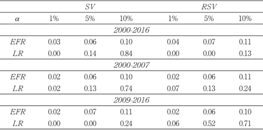
Table 4 shows the results of EFR, -values of the Kupiec LR test ( ) for the VaR forecasts of all the investigated time periods at a =1%, 5%, 10%. For a =10% at the 10% significance level, the estimates of EFR are not signifi-
cantly different from the corresponding probability a, which imply that the models are robust to predict the 10% VaR forecasts. In the RSV model, the null hypothesis that =a is rejected for a =1% and a= 5% even at the 10% significance level during the long time period of years 2000-2016, but not rejected at the 5% significance level in the cases of 2000-2007 and 2009-2016.
In contrast, although the for a= 5% of the years 2000-2016 suggests a superior performance of the SV model, the RSV model outperforms the SV model in most other cases of a =1% and a =5% at the 5% significance level.
It is also noticeable that the values of EFR are more inclined to rise for 2000- 2016 than for 2000-2007 and 2009-2016 due to the shaky financial markets of the year 2008 as shown in Figure 1.
The results of evaluation criteria (a) are summarized in Table 5.
Generally, the lower (a) indicate superior predictive ability of the RSV model for 2000-2007 and 2009-2016. On the other hand, the SV model is more suitable when the time span is expanded to 2000-2016.
Table 6 computes the loss functions MSE and QLIKE for the models. The
Table 4. Results for VaR
a 1% 5% 10% 1% 5% 10%
0.03 0.06 0.10 0.04 0.07 0.11
0.00 0.14 0.84 0.00 0.00 0.13
0.02 0.06 0.10 0.02 0.06 0.11
0.02 0.13 0.74 0.07 0.13 0.24
0.02 0.07 0.11 0.02 0.06 0.10
0.00 0.00 0.24 0.06 0.52 0.71
SRK (Hansen and Lunde (2005)) described as equation (15) is used as the proxy of latent volatility. The results of Table 6, which are in agreement with those of Table 5, state that the RSV model is more capable than the basic SV model for 2000-2007 and 2009-2016, but does not improve in predictive ability for 2000-2016.
5. Conclusion
This paper estimates the one-day-ahead VaR and ES forecasts for the S&P500 stock index, where latent volatilities are estimated by using the SV and RSV models. Observations of different time spans are chosen to investi- gate the model fitting.
Empirical studies show that the RSV model holds the advantage of describ- ing the biases of RVs due to non-trading hours and MMN, whereas this model does not always improve the predictive performance with respect to different time spans. Consequently, on the subject of the investigated stock index, RSV model fits data of short time spans better, while SV is more appropriate for the long time span.
Table 6. MSE and QLIKE
0.56 0.62 0.22 0.14 4.20 0.91
0.04 0.05 0.20 0.12 0.09 0.05
Table 5. Results for ES
a 1% 5% 10% 1% 5% 10%
0.19 0.25 0.23 0.29 0.30 0.26
0.26 0.19 0.17 0.25 0.14 0.14
0.31 0.26 0.20 0.31 0.21 0.18
Appendix A. Generation Algorithm for RSV Model
Substitute a ≡ -m, s ≡exp(m/2), ≡ξ +m into (5) ‒ (7), such the RSV model could be equivalently expressed as
(A1)
(A2)
(A3)
In the light of the work discussed in Omori and Watanabe (2008), this speci- fication will facilitate the generation steps through generating the latent a instead of on the condition that r ≠0.
Provided that the prior distributions of parameters are the following:
(f +1)/2 follows a beta distribution which ensures the stationarity assumption that |f|<1. (a/2, b/2) denotes an inversed gamma distribution with shape parameter a/2 and scale parameter b/2.
Given the prior distributions, samples of the parameters and latent volatili- ties can be drawn recursively from the respective posterior distributions via MCMC-based Bayesian method as follows.
( )
exp / 2 ,
t t t
R = a e
1 ,
t t t
a+ =fa +η
t t t,
x = +c a +u
η
η η
s rs s
η rs s s
s
∼ =
2 2
2
0
( , ), 0 .
0 0
e e
t
t e
t u
e N u
0Σ Σ
0 0
0 0 0 0
0 0 0 0
2
0 0
2
2 2
( , ), ( 1) / 2 ( , ),
( 1) / 2 ( , ), ( / 2, / 2),
( , ), u ( u/ 2, u/ 2).
N Beta a b
Beta a b IG
N IG
f f
r r η η η
ξ ξ
m m s f
r s a b
ξ m s s a b
+ +
A.1 Generation of θ (1) Generation of f
The conditional posterior density of f is p(f|m, r, sη2, a, R)
(A4)
where
(A5)
(A6)
The Metropolis-Hastings (MH) algorithm is applied since the samples of f are not easy to obtain from this conditional posterior density of (A4).
Specifically, the candidate f* is generated from (-1,1)(mf,sf2) in consideration of the restriction that |f|<1,where ( , )(m,s2) represents a truncated nor- mal distribution within the interval( , ). Given the current value f and accept f* with probability
(A7)
(2) Generation of G
Let G represents the 2×2 variance-covariance matrix of and η,
(A8)
1 1 2
2 2
2 1 1 1
2 2 2
exp( / 2)
(1 )
( ) 1 exp
2 2 (1 )
T
t t e t t
t η R
η η
a fa rs s a
p f f f a
s s r
- -
= +
- - - -
∝ - - - -
∑
0 0
2
1 1 2
2
( )
(1 ) (1 ) 1 exp ,
2
af bf f
f
f f f f m
s
- - -
∝ + - - -
1 1
1 1
2 2 1 2
1 2
exp( / 2) ,
T
t e t t t
t
T t t η R
f
a rs s a a
m r a a
- -
= +
-
=
- -
= +
∑
∑
2 2
2
2 2 1 2
1 2
(1 )
T .
t t f η
s r
s r a -a
=
= -
+
∑
0 0
0 0
1 1
* * *2
1 1 2
(1 ) (1 ) 1
, 1 .
(1 ) (1 ) 1
a b
a b
min
f f
f f
f f f
f f f
- -
- -
+ - -
+ - -
2
2 ,
e e
e
η
η η
s rs s rs s s
=
G
The logarithm of conditional posterior density about G is
(A9)
where
(A10)
(A11)
(A12)
Generate the candidate matrix G*-1~ (G1, 1), where ( , ) denotes a Wishart distribution with parameters ( , ), and accept it with probability
(A13)
If G*-1 is accepted, new draws of s*2, r*, sη*2 are obtained from G* and there- fore m*= s*2; else, samples will stay as the previous s2, r, s2η, m.
(3) Generation of ξ
The conditional posterior distribution of ξ is Gaussian with mean mξ1 and vari- ance sξ21 where
(A14)
(A15)
Generate ξ~ (mξ1,sξ21).
2 2 2
1
2 2
1 1
1
1
log ( , , ) log 1 log
2 2 exp( )
3 1
log ( ),
2 2
( ) T
e
e T
const R
tr
η
η
a f
p f s s
s s a
ν - -
= - - - - -
- + -
G a R
G G G
1 0 T 1,
ν =ν + -
1
1 1
1 0
1
,
T t t t
-τ τ
- -
=
= +
∑
′G G
1
exp( / 2)
t t .
t
t t
R a
τ a+ fa
-
= -
2 2 2
1
2 2
* *
2 2 2
* * 1
2 2
(1 )
exp 2 2 exp( )
,1 .
(1 )
exp 2 2 exp( )
T e
e T
T e
e T
R min
R
η
η
η
η
s s f a
s s a
s s f a
s s a
-
- -
-
- -
0 0
1
0
2 2
1
2 2
( )
,
T
t t u
t
u
x h T
ξ ξ
ξ
ξ
s s m
m s s
= - +
= +
∑
0 1
0
2 2
2
2 u 2.
T u ξ ξ
ξ
s s s
s s
= +
(4) Generation of s2u
It is also straightforward to generate s2 from the conditional posterior distri- bution (a1/2,b 1/2) where
(A16)
(A17)
A.2 Generation of h
Since the existence of high autocorrelation in the latent variables a, using sin- gle-move sampler, where only one a is generated at one time from full conditional distribution given all the other parameters, may bring about inef- ficient MCMC samples, this paper applies block sampler developed by Omori and Watanabe (2008) to improve the generation efficiency.
Equation (A18) shows the operation of how to divide (a1, a2, …, a ) into +1 blocks by selecting knots randomly in accordance with Shephard and Pitt (1997):
(A18)
where ( ) rounds to the nearest integer number and is a uniformly distributed random number in the interval (0, 1).
Suppose that there are m elements a( )=(a+1, a+2, …, a+ )′ included in the -th block. Given as and a+ +1, generating the normalized η(i)=(η, η +1, …, η + +1)′, which are easier to work with, is equivalent to generate the depen-
dent (a+1, a+2, …, a+ ) due to equation (A2).
The logarithm of joint conditional posterior density of η( ) (ignore the con- stant term) is
(A19)
where
1 0 ,
u u T
a =a +
( )
1 0
2 1
.
T
u u t t
t
x h
b b ξ
=
= +
∑
- -{
( ) / ( 2) ,}
1, 2, , ,i i
k =int T× +i U K+ i= K
(
( ) 1)
12 1 2log , , , , , , , , ,
2
s m i
s s m s s m s s m t
t s
f R R x x L
η
a a η
s
+ -
+ + + +
=
= -
∑
+
η θ
(A20)
(A21)
(A22)
(A23)
Consider that is a continuously differentiable function of a, a ( ×1) vec- tor d=( +1, +2, …, + )′ is the first derivatives of and a positive definite (m×m) matrix is -1 times the matrix of second derivatives of with respect to a. Let ^, d^ and Q^ represent , d and Q evaluated at a( )=a^( ), respectively. Approximate log (η( )|⋅) with a second-order Taylor expansion around the mode η^( )(or, equivalently, around a^( )):
(A24)
where (η( )|⋅) is the proposal density function and
2 2 1
1
1
1 ( ) , ,
2
, ,
s m
t s m s m
t s s m
t t s
l s m T
L
l s m T
η
a fa
s
+
+ + +
= + +
= +
- - + <
= + =
∑
∑
2 2
2 2
( ) ( )
log ( , , ) ,
2 2 2
t t t t t
t t t
t u
R x c
l f R X a m a
s s
- - -
≡ aθ = - - -
rs s aη fa a
m = - + - <
=
1
( 1 ) exp( / 2), ,
0, ,
e t t t
t
t T t T
2 2
2 2
(1 ) exp( ), ,
exp( ), .
e t
t
e T
t T t T
r s a
s s a
- <
=
=
(
( ) 1)
logf ηi a as, s m+ + ,Rs,,Rs m+ , ,xs,xs m+ , θ
η
η
σ η
σ η
α α
+ −
′
= =
′
= + −
=
+ + +
≅ − + + ∂ −
∂
∂
+ − ′ −
∂ ∂
′ ′
= − + + − − − −
≡
∑
∑
( ) ( )
( ) ( )
1
2 ( ) ( )
2 ( )
2
( ) ( ) ( ) ( )
( ) ( )
1
2 ( ) ( ) ( ) ( ) ( ) ( )
2
( )
1
1 ( )
2
1( )
2
1 1
( ) ( ) (
2 2
log ( , , , ,
( )
)
i i
i i
s m
i i
t i
t s
i i i i
i i
s m
i i i i i i
t t s i
s s m s s m
L L
E L
L
g R R
d Q
η η
η η
η η η
η η η η
η η
α α α α α α
η , ,xs,xs m+ , θ), ˆ
ˆ
ˆ ˆ ˆ ˆ ˆ
ˆ
ˆ ˆ
ˆ
ˆ η
η
σ η
σ η
α α
+ −
= ′ =
′
= + −
=
+ + +
≅ − + + ∂ −
∂
∂
+ − ′ ∂ ∂ −
′ ′
= − + + − − − −
≡
∑
∑
( ) ( )
( ) ( )
1
2 ( ) ( )
2 ( )
2
( ) ( ) ( ) ( )
( ) ( )
1
2 ( ) ( ) ( ) ( ) ( ) ( )
2
( )
1
1 ( )
2
1( )
2
1 1
( ) ( ) (
2 2
log ( , , , ,
( )
)
i i
i i
s m
i i
t i
t s
i i i i
i i
s m
i i i i i i
t t s i
s s m s s m
L L
E L
L
g R R
d Q
η η
η η
η η η
η η η η
η η
α α α α α α
η , ,xs,xs m+ , ),θ
ˆ
ˆ
ˆ ˆ ˆ ˆ ˆ
ˆ
ˆ ˆ
ˆ
ˆ η
η
σ η
σ η
α α
+ −
′
= =
′
= + −
=
+ + +
≅ − + + ∂ −
∂
∂
+ − ′ −
∂ ∂
′ ′
= − + + − − − −
≡
∑
∑
( ) ( )
( ) ( )
1
2 ( ) ( )
2 ( )
2
( ) ( ) ( ) ( )
( ) ( )
1
2 ( ) ( ) ( ) ( ) ( ) ( )
2
( )
1
1 ( )
2
1( )
2
1 1
( ) ( ) (
2 2
log ( , , , ,
( )
)
i i
i i
s m
i i
t i
t s
i i i i
i i
s m
i i i i i i
t t s i
s s m s s m
L L
E L
L
g R R
d Q
η η
η η
η η η
η η η η
η η
α α α α α α
η , ,xs,xs m+ , θ), ˆ
ˆ
ˆ ˆ ˆ ˆ ˆ
ˆ
ˆ ˆ
ˆ
ˆ
(A25)
(A26)
(A27)
(A28)
(A29)
(A30)
(A31)
(A32)
The expectations are taken with respect to ʼs conditional on aʼs. Hence
2
1 1 1
2 2 2
1
2
1 ( )
2 2
( ),
t t t t t t t t
t
t t t t t t
t t
t u
L R R R
d
x c
m m m m m
a s s a s a
a k a s
- - -
-
∂ - - ∂ - ∂
= = - + + +
∂ ∂ ∂
+ - - +
1 2
2 2 3
3 3
0 0
0 0 ,
0 0
s s
s s s
s s
s m
s m s m
A B
B A B
Q B A
B
B A
+ +
+ + +
+ +
+
+ +
=
1 exp , ,
2 2
0, ,
e t t t
t t
t T t T
η
rs f a fa a
m s
a
- + + - <
∂ =
∂ =
1
1
0, 1,
exp , 1,
2
t
e t
t
t t
η
ma rs a
s
-
-
=
∂∂ = >
f a fa sη
k a = + - = + <
2
( 1 ) / , ,
( )
0, ,
t t
t
t s m T otherwise
2 2
2 2
1
2 2 2
1
1 1 1 1
2 ( ),
t
t
t t
t
t t
t t u
A E L a
m m k a
a a
s s s
- -
∂
= -
∂
∂ ∂
= + ∂ + ∂ + + ′
2
1 1
2
1 1 1
1 t t ,
t
t t t t t
B E L m m
a a s a a
- -
- - -
∂ ∂ ∂
= - ∂ ∂ = ∂ ∂
2
2, ,
0 ( )
, .
t
t s m T otherwise
η
f k a s
= +
′ = <
the logarithm of proposal density function log (η( )|⋅) can be written as
(A33)
where ^ and ^ are values that and evaluated at a =a^ .
(1) Generation of η^(i)
Omori and Watanabe (2008) proposed to apply the Kalman filter (Anderson and Moore (1979), de Jong (1991)) and disturbance smoother (Koopman (1993)) to the linear Gaussian state space model to find the posterior modes of η^( ) and a^( ). This segment explicates the computation procedures by iterating the following algorithm several times until η^( ) converge to the posterior modes.
For = +1, …, + : Step 1. Initialize a^ .
Step 2. Compute ^ , ^ , ^ at a =a^ . Step 3. Calculate the following variables:
(
( ) 1)
logg ηi a as, s m+ +,Rs,,Rs m+ , ,xs,xs m+ , θ
1 2 2
1
2
1 1
1 2
1 ( )
2
1 ( ) 2 ( )( ) ,
2
s m s m
t t t t
t s t s
s m s m
t t t t t t t t
t s t s
L d
A B
η
η α α
σ
α α α α α α
+ − +
= = +
+ +
− −
= + = +
= − + + −
− − + − −
∑ ∑
∑ ∑
ˆ ˆ ˆ
ˆ ˆ ˆ ˆ ˆ
1 2
1
, 1,
, 2, , ,
t t
t t t
A t s
E A E B-- t s s m
= +
= - = + +
t t,
F = E
1 1
0, 1, 1,
, 2, , ,
t t t
t s s m
M B F−− t s s m
= + + +
= ˆ = + +
( ) 1
1 1
, 1,
, 2, , ,
t
t j
t t t t
d t s
b d M F b−− − t s s m
= +
= − = + +
ˆ ˆ
1
1 1,
t t F Mt t t
γˆ =αˆ + − +αˆ+
Step 4. The linear Gaussian state space representation is given by
(A34)
(A35)
where I is a 2×2 identity matrix and
Step 4-a. Apply the Kalman filter to (A34) and (A35), and generate the series { }= +1+ and { }= +1+ recursively:
(A36)
(A37)
where
Step 4-b. Compute the sequences { }=+ -1 and { }=+ -1 in succession by backward starting based on the disturbance smoother method:
(A38)
(A39)
Then
1 ,
t t t t
yˆ =γˆ +E b−
t t t t t,
yˆ =Zα +Gυ
1 ,
t t t t
a+ =fa +Hυ
. . . ( , ),
t i i d N 0I υ
1 1 1
1 1
1 , , , 0,
t t t t t t t t
Z = +F M- +f G =F- F M- +sη H = sη
1
0, ,
, 1, , 1,
t
t t t
t s a+ fa Kz t s s m
=
= + = + + -
2 1
, ,
, 1, , 1,
t
t t t t
t s
P P L t s s m
sη + f
=
=
+ ′ = + + -
H J
2 1
, , ( ) ,
, .
t t t t t t t t t t t t t t t
t t t t t t t
y Z D Z P K P Z D
L K Z K
ζ α φ
φ
′ ′ −
= − = + = +
= − = −
GG H G
J H G
ˆ
1 1
0, ,
, 1, , ,
t
t t t t t
t s m r- Z D-z L r t s m s
= +
= + = + -
1 2 1 2
0, ,
, 1, , .
t
t t t t
t s m U- Z D- L U t s m s
= +
=
+ = + -