再突入機体周りのプラズマ流れと通信途絶に関する数値解析的研究

(1)

再突入機体周りのプラズマ流れと通信途絶に関する数値解析的研究

鄭, 旻錫

https://doi.org/10.15017/1931915

出版情報：Kyushu University, 2017, 博士（工学）, 課程博士バージョン：

権利関係：

(2)

Radio Frequency Blackout for Reentry Vehicle

by

Minseok Jung

Department of Aeronautics and Astronautics, Kyushu University, Fukuoka, Japan

February, 2018

(3)

1 Introduction 1

1.1 Background . . . 1

1.2 RF Blackout . . . 2

1.3 Previous Studies of RF Blackout . . . 3

1.4 Objectives . . . 5

1.5 Thesis Overview . . . 6

2 Flow Characteristics and Modeling 7 2.1 Thermal Nonequilibrium . . . 7

2.2 Chemical Nonequilibrium . . . 8

2.3 Flowfield Equations . . . 8

2.3.1 Mass conservation . . . 9

2.3.2 Momentum conservation . . . 9

2.3.3 Energy conservation . . . 10

2.4 Chemical Reaction Model . . . 12

2.4.1 Reaction Rate . . . 12

2.4.2 Reaction Model . . . 13

2.5 Thermodynamics Model . . . 17

2.5.1 Thermodynamics Properties . . . 17

2.5.2 Equation of State . . . 18

2.6 Transport Properties . . . 20

2.6.1 Collision Cross Section . . . 20

2.6.2 Viscosity . . . 22

2.6.3 Thermal Conductivity . . . 23

2.6.4 Electrical Conductivity . . . 25

2.6.5 Diﬀusion . . . 25

2.6.6 Summary of Transport Properties . . . 27

2.7 Internal Energy Exchange Model . . . 28

2.7.1 Translational-Rotational Energy Exchange . . . 29

2.7.2 Translational, Rotational-Vibrational Energy Exchange . . . 29

2.7.3 Translational-Electron Energy Exchange . . . 32

2.7.4 Rotational-Electron Energy Exchange . . . 32

2.7.5 Vibrational-Electron Energy Exchange . . . 33

2.7.6 Vibrational and Rotational Energy Losses Due to Dissociation Reaction . . . 33

2.7.7 Electron Energy Loss Due to Dissociation and Ionization Reactions 34 2.8 Summary of Governing Equations . . . 34

3 Numerical Procedure 36 3.1 Discretization . . . 36

3.2 Numerical method . . . 38

3.3 Inviscid flux . . . 41

3.3.1 SLAU2 Scheme . . . 42

3.3.2 MUSCL Approach . . . 43 i

(4)

3.4 Viscous flux . . . 45

3.5 Time Integration . . . 47

3.5.1 Implicit Scheme . . . 48

3.5.2 Point Implicit Method . . . 49

3.5.3 LU-SGS Method . . . 49

3.6 Electron Energy Equation . . . 53

3.7 Boundary Conditions . . . 57

3.8 Grid System . . . 58

3.9 Other Implementations . . . 59

3.9.1 Local Time Stepping . . . 59

4 Electromagnetic Wave Modeling 60 4.1 Governing equations . . . 60

4.2 Modeling . . . 61

4.3 Numerical method . . . 61

4.4 Transmitting antenna . . . 64

4.5 Mapping process . . . 64

4.6 Boundary conditions . . . 64

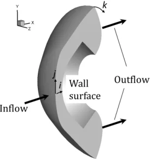
5 Results and Discussion 66 5.1 Analysis Objects . . . 66

5.1.1 Orbital Reentry Experiment . . . 66

5.1.2 Atmospheric Reentry Demonstrator . . . 68

5.2 Validation of Flowfield Simulation Model with Experimental Results of OREX . . . 72

5.3 Validation of CFD-FD2TD Combined Method with Experimental Re- sults of ARD . . . 76

5.3.1 Eﬀect of Angle of Attack . . . 76

5.3.2 Eﬀect of Catalytic Recombination . . . 83

5.3.3 Uncertainty in chemical reaction rate model . . . 88

6 Conclusion 96 A 100 A.1 Jacobian Matrices of Inviscid Term . . . 100

A.2 Jacobian Matrix of Source Term . . . 103

References 105

ii

(5)

1.1 Schematic diagram of causes of RF blackout . . . 2

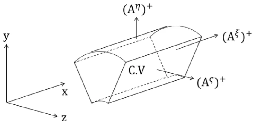
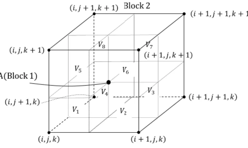
3.1 Control volume . . . 37

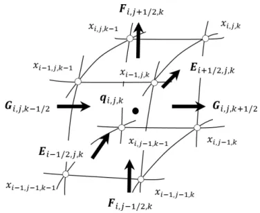
3.2 Cell system . . . 38

3.3 Boundary conditions. . . 57

3.4 Schematic of interpolation. . . 59

4.1 Typical computational grid of FD2TD method . . . 62

4.2 Yee cell . . . 62

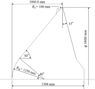
5.1 Configuration of the OREX . . . 67

5.2 Locations of the electro-static probes . . . 67

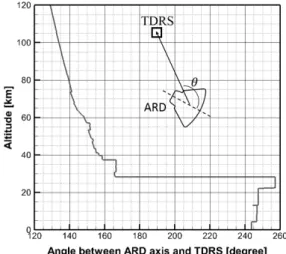
5.3 Configuration of the ARD . . . 69

5.4 Location of TDRS on ARD . . . 69

5.5 Angle between the ARD axis and TDRS . . . 70

5.6 Windows in which the TDRS is visible at each altitude . . . 71

5.7 Computational grid systems of the OREX at an altitude of 84.01 km . 72 5.8 Temperatures on the stagnation line at an altitude of 84.01 km for OREX 73 5.9 Mole fractions on the stagnation line at an altitude of 84.01 km for OREX 73 5.10 Saturation ion current at probes 1 - 5 of OREX . . . 75

5.11 Computational grid systems of ARD for the axisymmetric model and the three-dimensional model . . . 76

5.12 Distributions of translational temperature at an altitude of 85 km around the ARD vehicle for the axisymmetric model and the three-dimensional model . . . 77

5.13 Distributions of electron temperature at an altitude of 85 km around the ARD vehicle for the axisymmetric model and the three-dimensional model . . . 77

5.14 Distributions of electron number density at an altitude of 90 km around the ARD vehicle for the axisymmetric model and the three-dimensional model . . . 78

iii

(6)

dimensional model . . . 81 5.20 Behavior of electromagnetic waves at an altitude of 85 km around the

ARD vehicle with the results of the axisymmetric model and the three- dimensional model . . . 81 5.21 Behavior of electromagnetic waves at an altitude of 60 km around the

ARD vehicle with the results of the axisymmetric model and the three- dimensional model . . . 82 5.22 Comparison of signal losses for investigating the eﬀect of angle of attack 82 5.23 Computational grid systems of ARD at an altitude of 85 km for NCW

and FiCW . . . 83 5.24 Distributions of electron number density at an altitude of 90 km around

the ARD vehicle for NCW and FiCW . . . 84 5.25 Distributions of electron number density at an altitude of 85 km around

the ARD vehicle for NCW and FiCW . . . 85 5.29 Behavior of electromagnetic waves at an altitude of 90 km around the

ARD vehicle with results of NCW and FiCW . . . 86 5.30 Behavior of electromagnetic waves at an altitude of 85 km around the

ARD vehicle with results of NCW and FiCW . . . 86 5.31 Behavior of electromagnetic waves at an altitude of 60 km around the

ARD vehicle with results of NCW and FiCW . . . 87 5.32 Comparison of signal losses for investigating the eﬀect of catalytic re-

combination . . . 87 5.33 Computational grid systems of ARD for parametric study . . . 89 5.34 Distributions of electron number density in case 1-9 at an altitude of 85

km around the ARD vehicle . . . 90 5.35 Distributions of electron number density in case 1-9 at an altitude of 77

km around the ARD vehicle . . . 91 5.36 Distributions of electron number density in case 1-9 at an altitude of 70

km around the ARD vehicle . . . 92 5.37 Behavior of electromagnetic waves in case 1-9 at an altitude of 85 km

around the ARD vehicle . . . 93 5.38 Behavior of electromagnetic waves in case 1-9 at an altitude of 77 km

around the ARD vehicle . . . 94 5.39 Comparison of signal losses with parametric study . . . 95

iv

(7)

2.1 Chemical reactions . . . 16

2.2 Chemical species data . . . 18

2.3 Curve-fit constants forσ_e,s . . . 32

2.4 Curve-fit constants forτs . . . 33

2.5 Dissociation energy and ionization energy . . . 34

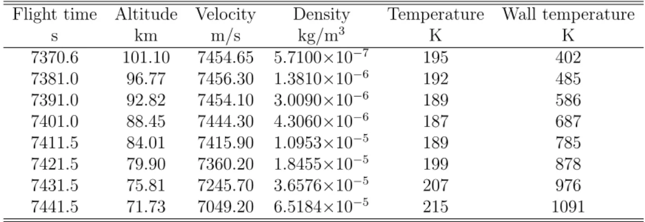
5.1 Computational conditions for the OREX . . . 68

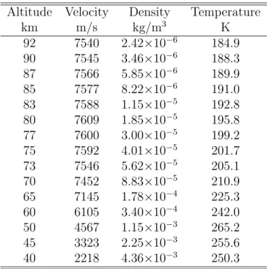
5.2 Computational conditions for the ARD . . . 71

5.3 Uncertainty factors of forward reaction rates . . . 88

v

(8)

B = magnetic flux density vector, T c = speed of sound, m/sec

C = mass fraction

C_v = specific heat at constant volume, J/(kg · K) C_p = specific heat at constant pressure, J/(kg · K) D = effective diffusion coefficient, m²/sec

D = binary diﬀusion coeﬃcient, m²/sec D = electric flux density, C/m²

e = energy per unit mass, J/kg, or electric charge, C E = internal energy, J/m³

E = electric field vector, V/m

ED = dissociation energy per unit mass, J/kg E_I = ionization energy per unit mass, J/kg F = vector of inviscid terms

Fv = vector of viscous terms g = relatively velocity, m/sec

h = enthalpy, J/kg

∆h⁰ = enthalpy of formation, J/kg H = magnetic field vector, A/m I = identity matrix

Js = Jacobian, or diﬀusion flux of species s, kg/(m² ·sec) J = current density vector, A/m²

k = Boltzmann constant, J/K, or reaction-rate coeﬃcient, m³/(mole·sec) K^eq = equilibrium constant

m = mass, kg

˙

m = mass flux, kg/(m²·sec) M = molar mass, kg/mole n = number density, 1/m³ nm = number of molecular species ns = number of species

p = pressure, Pa

q = heat flux, W/m²

Q = internal energy-exchange rate, W/m³ Q = vector of conservative variables R = gas constant, J/(kg · K)

R = residual vector

S_int = internal energy-exchange rate, W/m³

t = time, sec

T = temperature, K

u = velocity, m/sec

v = velocity, m/sec, reaction rate, mole/(m³ · sec) V = volume, m³, diﬀusion velocity, m/sec

˙

w = mass-production rate, kg/(m³ · sec)

vi

(9)

X = mole fraction α = degree of ionization

γ = specific heat ratio, or reduced velocity δ_ij = Kronecker delta

εr = relative permittivity

ε₀ = permittivity in free space, N/V²

θ = angle

Θ = characteristic temperature, K λ = thermal conductivity, W/(K · m) µ = molecular viscosity, N ·sec/m² µ0 = permeability in free space, N/A² ν = collision frequency, 1/sec

ν_s,r = stoichiometric coeﬃcient of reaction r of species s ξ,η,ζ = direction in computational space

πΩ = collision cross section, m² ρ = density, kg/m³

σ = conductivity, S/m, or eﬀective collision cross section, m² σ_i,j = diﬀerential scattering cross section for species i and j σSB = Stefan-Boltzmann constant, W/(K⁴·m²)

τ = relaxation time, sec, stress, N/m²

χ = angle of deflection, or electric susceptibility ωp = plasma angular frequency, rad/sec Subscripts

av = mass-averaged

B = magnetic

b = backward

CFL = Courant-Friedrichs-Lewy condition D = dissociation, or Debye

e = electron

ex = electronic excitation

E = electric

f = forward

I = ionization

in = inflow

int = internal

L = left

M = molecular

R = rotation, or right ref = reference

rot = rotation

s = species

T = translation

tr = translation

V = vibration

v = viscous

vib = vibration

vii

(10)

1/2 = cell interface

viii

(11)

Introduction

1.1 Background

Our curiosity about the universe continues unchanged from the past to the present.

Furthermore, its interest has been increasing toward the future with the rapid development of science and technology. In recent years, space development is indispensable not only to satisfy curiosity, but also to solve problems related to human survival ac- companying population increase and energy depletion. There is an increasing interest in the mission that requires a sample return after the exploration of asteroid and the reentry into the atmosphere for recovery of supplies and personnel from the Interna- tional Space Station (ISS). Hayabusa (MUSES-C) spacecraft of the Japan Aerospace Exploration Agency (JAXA) successfully returned into the Earth from asteroids in 2010, and Hayabusa 2 which is a successor of Hayabusa has been launched on 3 De- cember 2014 for the purpose of sample return from C-type asteroids. As a development of Kounotori (H-II Transfer Vehicle, HTV) which is a currently operating space station transfer vehicle, JAXA is developing a type of HTV which has a reentry capsule, called HTV-R [1]. This vehicle is very important not only for recovering supplies from the ISS but also for establishing essential technologies for future manned space activities.

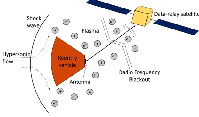
In order to safely return the spacecraft, the entry, descent, and landing (EDL) approach technology is mightily important. In the EDL approach, it is necessary to assess the position of the reentry vehicle accurately and to recover the vehicle quickly after its landing/splashing down during a reentry mission. For the assessment of position, it is important to maintain communication between the reentry vehicle and ground station. The Global Positioning System (GPS) and Iridium satellite network with electromagnetic waves are used for communication between the reentry vehicle and ground station. However, a strong shock wave forms in front of the reentry vehicle because the reentry speed of vehicle is exceeding 7 km/s. In the shock layer, the air is dissociated and ionized due to strong aerodynamic heating, and plenty of ions and electrons are generated around the reentry vehicle. The electromagnetic waves used for telecommunication, navigation, guidance, and control are attenuated and reflected by a plasma layer around the reentry vehicle. The ground station and data relay satellite therefore cannot receive the electromagnetic waves, and this phenomenon is called radio frequency (RF) blackout [2–4]. The RF blackout that means the cutoﬀ of communication between the reentry vehicle and the ground station disturbs the accurate assessment of the position of reentry vehicle in real time. Figure 1.1 shows a schematic

1

(12)

diagram of causes of RF blackout around the reentry vehicle.

Fig. 1.1: Schematic diagram of causes of RF blackout

1.2 RF Blackout

The RF blackout has been observed in many reentry flight. For instance, Mercury, Gemini, and Apollo spacecraft experience several minutes of RF blackouts. In Gemini 2, four minutes of RF blackout was observed. In addition, Apollo 13 command mod- ule underwent the RF blackout about six minutes, and it was longer than had been predicted. For the Soyuz Transport Modified Anthropometric (TMA) reentry vehicle, RF blackout about 10 minutes is observed. RF blackout also occurs when the vehicle enters a planetary atmosphere at hypersonic velocity. For the Mars Pathfinder spacecraft, communications with the earth were lost for an approximately 30 second period during the descent phase into Martian atmosphere on July 4, 1997 [5]. The National Aeronautics and Space Administration (NASA) Deep Space Network (DSN) 70-m antenna located in Madrid, Spain received the emitted signal frequency of 8.43 GHz in the one-way tracking mode. The possibility that the interaction of the heat shield with the Martian atmosphere generated ions was raised among the several possible explana- tions. The flight profile of Pathfinder during the blackout period was used to estimate electron density employing an aerothermodynamic program [6]. The estimated electron number density exceeded the critical electron density required for blackout at 8.4 GHz (X-band) at least during the first 20 seconds. In many reentry flight test, such as Radio Attenuation Measurement C II (RAM C II) [7, 8] of NASA, Orbital Reentry Experiment (OREX) [9] of JAXA and Atmospheric Reentry Demonstrator (ARD) [10]

of European Space Agency (ESA) flight tests, the RF blackout also has been observed.

In addition, the blackout problem is an important issue both for safety and catastrophe

(13)

analysis. In the Space Shuttle Colombia disaster, it was diﬃcult to find the cause of disaster because of the RF blackout.

1.3 Previous Studies of RF Blackout

Several techniques for mitigation of the RF blackout problem have been proposed by various researchers, such as the magnetic window [11–13], electrophilic fluid injection [14,15], E×B layer [16–18], resonant transmission [19], time varying magnetic field [20], electron acoustic wave transmission [21], wave frequency modification and aerodynamic shape modification. The magnetic window mitigation scheme is to apply an external magnetic field to the plasma layer for converting the free space radio wave to a whistler wave in the plasma. Electrophilic injection uses an electrophilic substance injected into the fluid to decrease the plasma density. In the Gemini 3 mission [22], water injection as an electrophilic substance was used. E × B layer approach accelerates the plasma past the antenna by applying an E × B layer near the antenna, and the density of the accelerated plasma will decrease to satisfy mass conservation. A window in the plasma layer can be generated by the E × B layer, and electromagnetic wave can propagate passing through the plasma layer. Resonant transmission scheme is to use resonance with a surface wave to enhance transmission in the plasma layer.

Time varying magnetic field approach uses the Hall effect. A pulsed current generates a rising magnetic field. The electrons are expelled across the field due to the time varying magnetic field, and the plasma density is decreased periodically. Electron acoustic wave transmission approach is to transmit signals across the plasma layer by employing electron acoustic wave transmission. Belov et al. [23] investigated an aerodynamic shaping techniques using the antennas in special small containers ahead of a blunt nose vehicle. Takahashi et al. [24, 25] suggested that a membrane-aeroshell (inflatable) reentry vehicle can reduce RF blackout using its low ballistic coefficient and large projected area for deploying its flare aeroshell in orbit. In the design process of reentry vehicles, the possibility of communications between the reentry vehicle and ground station must be investigated. However, it is difficult to accurately reproduce the environment in which RF blackout occurs by using ground testing facilities, such as hypersonic wind tunnels, arc-heated wind tunnels or inductively-coupled-plasma wind tunnels. Numerical simulations has been effectively applied with the recent remarkable development of computers and numerical schemes.

It is necessary to clarify the plasma flow and complex movement of electromagnetic waves around the reentry vehicle when estimating the possibility of RF blackout and signal loss. The possibility of communication during a reentry phase has been numerically investigated by several groups with many diﬀerent codes. Tran et al. [26]

numerically investigated the plasma density around the ARD using the computational fluid dynamics (CFD) method. Usui et al.[27] numerically investigated the RF blackout of a reentry vehicle by performing electromagnetic Particle-In-Cell (PIC) simulations [28]. They also examined the possibility of communication during RF blackout via whistler mode. Thoma et al. [13] numerically investigated the magnetic window with a horn antenna using the high density finite-diﬀerence time-domain (FDTD) PIC code LSP. As multi-fluid electromagnetic approach has been developed by several researchers [29–33], an application of multi-fluid electromagnetic approach to modeling RF blackout has been suggested. Visbal et al. [34] used a multi-fluid electromagnetic

(14)

approach to modeling radio communication blackout on an over-set mesh. Kundrapu et al. [35] numerically investigated the propagation of plane electromagnetic waves on to the surface of a reentry vehicle through the plasma layer via a magnetic window and the whistler wave conversion by using code USim [36–38].

Takahashi et al. [25, 39] proposed a numerical simulation method of RF blackout with CFD for plasma flow and the frequency-dependent finite-diﬀerence time-domain (FD2TD) method [40, 41] for electromagnetic waves. The FD2TD method is useful in predicting the behavior of electromagnetic waves in a frequency-dependent medium such as plasma, and has been used to determining the propagation of microwaves around a rocket plume [42] and that of electromagnetic waves in isotropic cold plasma [43]. Takahashi et al. [39] numerically investigated the possibility of communication for the ARD using a CFD-FD2TD combined method, and validated the model with measured signal loss data. In their numerical simulations, strong signal losses and RF blackout which was not observed in the flight test, were predicted at some altitudes although the predicted data were generally in good agreement with the trends of the measured data. The discrepancies might be caused by plasma flow around the ARD that was not precisely predicted. The flowfield around a reentry vehicle tends to be in a thermochemical nonequilibrium state. When investigating the RF blackout, it is necessary to construct the nonequilibrium flow accurately in order to predict the electron number density.

For investigating the flowfield around a reentry vehicle, an axisymmetric condition is often imposed on the flowfield to reduce the computational cost [25, 39]. Most of the reentry vehicle has been flown with a non-zero angle of attack, however an axisymmetric condition cannot reproduce an angle of attack. Unlike the typical numerical simulations around a reentry vehicle, such as the prediction of heat flux, it is necessary to evaluate the distribution of electron number density in the wake region when investigating the possibility of communications. Therefore, a three-dimensional flowfield model which can reproduce an angle of attack should be used, and its use may change the formation of the plasma in the wake region for a reentry vehicle flight with a non-zero angle of attack.

In addition, wall catalytic recombination might contribute to formation of distribution of chemical species, especially electrons and ions, around the reentry vehicle.

Molecules that have passed through the shock wave go through various chemical reactions and become atoms or ions. When atoms directly reach the wall surface, depending on the material of the wall surface, diﬀused atoms may be captured on the wall surface and recombined to the molecule and released. In the case where the wall surface causes a recombination reaction, it is called that the wall surface is catalytic. Due to the catalytic eﬀect, when a recombination reaction occurs on the wall surface, since this reaction is an exothermic reaction, the reaction heat directly heats the wall surface.

Therefore, it is known that the catalytic effect greatly increases heat flux. The wall catalytic recombination is an important factor in the design of the thermal protection system of the reentry vehicle. From the design requirement to reduce the wall heating, wall materials of reentry vehicles are made of materials having as small a catalytic effect as possible. However, it is difficult to completely eliminate it, and it often has finite catalytic efficiency. The wall catalytic recombination have a great influence not only on heat flux but also on the formation of chemical species around the reentry vehicles. Therefore, the wall catalytic recombination should be considered properly.

(15)

Chemical reaction rates model has a direct eﬀect on the formation of chemical species around the reentry vehicle. There are various models for chemical reactions, and they have been proposed by several researchers [44–51]. However, there may be an inherent discrepancy with the true value when chemical reaction rate models are used for a wide temperature range because these models are based on experimental results obtained within certain temperature ranges. Uncertainty in chemical reaction rates model should be considered properly because it is necessary to predict accurately the plasma properties around the reentry vehicle when investigating the RF blackout.

1.4 Objectives

In the design and development process of reentry vehicles, the prediction of RF blackout must be evaluated. It is necessary to investigate the plasma flow, involving complex chemical reactions, and to analyze the attenuation and reflection of electromagnetic waves around the reentry vehicle in detail. The CFD-FD2TD combined method is powerful tool for investigating the plasma flow and electromagnetic waves around the reentry vehicle.

The main purpose of the present study is to construct the accurate prediction tool of RF blackout using the CFD-FD2TD combined method. It is important to clarify the plasma flow around the reentry vehicle. A lot of research has been done on the plasma physics and nonequilibrium phenomena, and thermochemical models of high- temperature gas have been developed. In the present study, the plasma flow around the reentry vehicle is numerically studied using CFD with various models. The FD2TD method is used to investigate the complex behavior of electromagnetic waves with the plasma properties obtained by the CFD model. In addition, several discussions are presented to accurately determine the flowfield in the present study.

It is important to investigate the distribution of electron number density in the wake region accurately when evaluating the possibility of communications. The three- dimensional model with a non-zero angle of attack is mainly used in the numerical study of plasma flow for accurate prediction of RF blackout. The axisymmetric model is also used for comparison with the results of the three-dimensional model. The eﬀect of angle of attack on the plasma properties and the evaluation of RF blackout are investigated around the reentry vehicle.

It is thought that the wall catalytic recombination aﬀects the generation of electrons in front of the reentry vehicle, and the formation of electrons in the wake region.

The non-catalytic wall (NCW) and finite-catalytic wall (FiCW) conditions are therefore employed to investigate the eﬀect of catalytic wall on the distribution of electron number density around the reentry vehicle and the prediction of RF blackout.

In the numerical simulations of RF blackout, the chemical reactions that mainly determine the generation of electrons should be treated carefully because they may have an inherent discrepancy with the true value. Therefore, it should be investigated how uncertainty in chemical reaction models aﬀects the formation of electrons around the reentry vehicle and the evaluation of RF blackout. A parametric study of the chemical reaction rates is performed to investigate the eﬀect of uncertainty in chemical reaction model in the present study.

(16)

1.5 Thesis Overview

The outline of the present thesis is denoted here. First, the background and the research objectives were discussed in the present chapter, Chapter 1.

In Chapter 2, the governing equations and models used to describe the flowfield are presented. In order to simplify the problem, we introduce some assumptions for the flowfield. Governing equations, i.e., The Navier-Stokes equations extended to thermochemical nonequilibrium and the equation of state, are constructed based on these assumptions. Transport properties and thermochemical nonequilibrium models, such as chemical reaction and internal energy transfer models, are presented.

Numerical simulation methods for the flowfield are mainly described in Chapter 3.

The governing equations are solved using a finite volume approach. The numerical fluxes of the flowfield equations are evaluated using proper schemes, respectively. The time integration is performed implicitly. The boundary conditions and the grid system are given. In addition, the NCW and FiCW conditions are presented.

Chapter 4 gives the governing equations, i.e., Maxwell’s equations, for describ- ing the behavior of electromagnetic waves. The mapping process to refer the plasma properties of the flowfield simulations is addressed. The FD2TD formulation for the numerical simulation of Maxwell’s equations is given. In the present FD2TD formulation, the complex relative permittivity is given assuming the first Drude dispersion.

The boundary condition for the electromagnetic waves is given in this chapter.

In Chapter 5, computational results of flowfield and electromagnetic waves for the reentry vehicles are described by using the numerical models presented in the previous chapters. The eﬀects of the angle of attack, catalytic recombination, and uncertainty in chemical reaction rate model on the evaluation of RF blackout, are discussed in detail.

The computational results are also compared with the actual flight data to validate the present numerical model.

Finally, some conclusions of the present study are described in Chapter 6.

(17)

Flow Characteristics and Modeling

2.1 Thermal Nonequilibrium

Molecules, atoms, ions, and electrons have some internal energy degrees of freedom, as follows:

1. Translational energy representing the magnitude of translational motion of particles

2. Rotational energy associated with the rigid rotational motion of molecules 3. Vibrational energy stretching the interatomic bonds constituting the molecule 4. Electronic excitation energy representing the state of an electron’s orbital sur-

rounding the nucleus (electronic excited state)

5. Electron energy representing the magnitude of translational motion of electrons (free electrons) jumping out of molecules or atoms by collision

When the particles follow the Maxwell-Boltzmann distribution, it is possible to define the temperature of each energy mode, translational temperatureT_tr, rotational temperature Trot, vibrational temperature Tvib, electron excitation temperature Tex

and electron temperature T_e. When suﬃcient inter-particle collisions are occurring, the energy exchange between the energy modes quickly proceeds so that each energy mode can be described at one temperature. This is called a thermal equilibrium state.

On the other hand, if the collision between the particles is not suﬃcient, it may become impossible to represent each energy mode at one temperature. This is called a thermal nonequilibrium state.

In the thermal nonequilibrium state, it is desirable that a detailed multi-temperature model which separates the temperature into translational (T_tr), rotational (T_rot), vibrational (Tvib), electron excitation (Tex) and electron temperature (Te) is introduced.

In this case, five energy equations are added to the equation system. It is required a notable attention to use those models because the physical data for internal energy exchange model, although have been developed, are partly lacking. In particular, the relaxation models between the electronic excitation and other energy modes have unclear points

7

(18)

In this study, the temperature is separated into four temperatures of translational, rotational, vibrational and electron temperature. However, it is assumed that the electron excitation temperature is equal to the electron temperature, and the translational, rotational and vibrational temperatures are common for all chemical species.

2.2 Chemical Nonequilibrium

Chemical reactions proceed at a finite rate, which is influenced by the frequency of collisions between particles. If the collisions between the particles are suﬃciently large, the chemical reaction rapidly reaches equilibrium, so it is determined by local temperature and density (or total pressure). On the other hand, if the collision between the particles is small, it will flow before the chemical reaction occur and will eventu- ally become a flow field without chemical reactions. Such flows are called chemically equilibrium flow and chemically frozen flow, respectively. On the other hand, when the characteristic time of the chemical reaction and the characteristic time of the flow are on the same order, the chemical reaction will occur while flowing. Such a flow is called chemical nonequilibrium flow.

In a flowfield around a hypersonic vehicle, chemical reactions such as dissociation and ionization occur in a high temperature region behind the shock wave, and chemical nonequilibrium appears. For this reason, the numerical simulation is performed assuming the chemical nonequilibrium flow in the present study.

2.3 Flowfield Equations

The present study assumes that the flow is laminar, steady and continnum. As the inflow gas, air is used. Based on these assumptions, flowfield equations are described in the present section. The flowfield around a reentry vehicle can be described by the total mass, momentum and total energy conservations. Additionally, the species mass, rotational, vibrational and electron energy conservations are added to the set of the equations in order to describe the thermochemical nonequilibrium flow.

In this study, single rotational and vibrational temperature are considered for all molecules. It is reported that the vibration-vibration energy relaxations are not small compared with the other contributions and the vibrational temperatures are not always equilibrated. However, in the present study, mole fractions of the charged molecules (such as N⁺₂, N⁺₂ and NO⁺) are expected to be smaller than those of the neutral molecules (N₂, O₂ and NO), and it is expected that separation of the vibrational temperature does not largely aﬀect the flow properties. Therefore, single rotational and vibrational temperature are used for simplicity and reduction of the computational cost in the present study.

The macroscopic equations can be derived from moments of the Boltzmann equation. Multiplying the average quantity per unit particle⟨φs⟩, the Boltzmann equation becomes

∂

∂t(n_s⟨φ_s⟩) + ∂

∂xj

(n_s⟨φ_su^j_s⟩)

=S(⟨φ_s⟩), (2.1) where “⟨ ⟩” represents the averaged value of a quantity, andn_s and v_s^j are the number density of species s and jth component of particle velocity, respectively. In addition,

(19)

S(⟨φs⟩) shows the rate of change by interactions among species.

2.3.1 Mass conservation

The mass conservation for species s can be obtained by taking φ_s = m_s in Eq.

(2.1). First, the mass density is written by, n_s⟨m_s⟩ = ρ_s, and the jth component of the thermal velocity is defined as follows:

C_s^j ≡u^j_s−u^j₀, (2.2)

where u^j₀ is the jth component of the mass-averaged velocity given by

u^j₀ =

∑ns s

ρ_su^j_s

∑ns s

ρ_s

. (2.3)

Thus, replacing the thermal velocity C_s^j by the diﬀusion velocity V_s^j, the mass conservation for species s is written by

∂ρs

∂t + ∂

∂x_j [ρ_s(

u^j₀+V_s^j)]

= ˙w_s, (2.4)

where ˙w_s represents the mass production rate due to collisions. The summation of Eq.

(2.4) over all the species yields

∂

∂t

∑ns s

ρ_s+ ∂

∂x_j [ _ns

∑

s

ρ_su^j₀+

∑ns s

ρ_sV_s^j ]

=

∑ns s

˙

w_s. (2.5)

Since

∑ns s

ρ_sV_s^j and

∑ns s

˙

w_s are zero by definition, we obtain the total mass conservation as follows:

∂ρ

∂t +∂(ρu^j₀)

∂x_j = 0, (2.6)

where

ρ =

∑ns s

ρ_s. (2.7)

2.3.2 Momentum conservation

The momentum conservation equation for the speciesscan be obtained by replacing the quantity φ_s with the momentum m_suⁱ_s. In this case, the production rate term S(⟨m_suⁱ_s⟩) is the interaction force due to collision of species F_int,sⁱ . The second term on the left hand side of Eq. (2.1) in identifying φ_s=m_su^j_s is expressed by

n_s⟨m_suⁱ_su^j_s⟩=ρ_s(

⟨uⁱ₀u^j₀⟩+⟨uⁱ₀C_s^j⟩+⟨C_sⁱu^j₀⟩+⟨C_sⁱC_s^j⟩)

=ρ_s(

uⁱ₀u^j₀+⟨C_sⁱC_s^j⟩)

. (2.8)

(20)

The viscous stress tensor τ^ij is defined as τ_s^ij ≡ −(

ρ_s⟨C_sⁱC_s^j⟩ −p_sδ^ij)

, (2.9)

where δ^ij is the Kronecker delta. The momentum conservation can be obtained as follows:

∂

∂t

(ρ_suⁱ_s) + ∂

∂x^j

(ρ_suⁱ₀u^j₀+p_sδ^ij)

−∂τ_s^ij

∂x^j =F_int,sⁱ . (2.10) In the same way as the total mass conservation, the total momentum conservation equation is obtained by summation over all the species:

∂

∂t (ρuⁱ₀)

+ ∂

∂x^j

(ρuⁱ₀u^j₀+pδ^ij)

− ∂τ^ij

∂x^j = 0. (2.11)

According to Hirschfelder, Curtiss and Bird [52], the viscous stress tensor is given by τ^ij =µ

(

∂uⁱ₀

∂x^j + ∂u^j₀

∂xⁱ −2 3

∂u^k₀

∂x^kδ^ij )

, (2.12)

where µis the viscosity for a gas mixture. Consequently, the total momentum conservation equation is expressed by

∂

∂t (ρuⁱ₀)

+ ∂

∂x^j

(ρuⁱ₀u^j₀+pδ^ij)

= ∂

∂x^j [

µ (

∂uⁱ₀

∂x^j +∂u^j₀

∂xⁱ )

−2 3µ∂u^k₀

∂x^kδ^ij ]

. (2.13)

2.3.3 Energy conservation

The energy conservation equation for speciessis obtained by taking⟨φ_s⟩=⟨₂¹m_suⁱ_suⁱ_s⟩+

⟨ϵ_int⟩, where the ⟨¹₂m_suⁱ_suⁱ_s⟩ and ⟨ϵ_int⟩ are the average densities of translational energy and internal energy of rotational, vibrational, electron and chemical energy mode, respectively. The density of translational energy is expressed as

⟨1

2m_suⁱ_suⁱ_s⟩= 1 2m_s

∑3 i

⟨uⁱ_suⁱ_s⟩, (2.14) where

⟨uⁱ_suⁱ_s⟩=⟨(

uⁱ₀+C_sⁱ)2

⟩=uⁱ₀uⁱ₀+⟨C_sⁱC_sⁱ⟩. (2.15) Hence, the energy becomes

n_s⟨1

2m_suⁱ_suⁱ_s⟩+n_s⟨ϵ_int⟩=ρ_s (1

2uⁱ₀uⁱ₀+1

2⟨C_sⁱC_sⁱ⟩+e_int,s )

=ρ_s (1

2uⁱ₀uⁱ₀+e_s )

, (2.16)

(21)

wherees represents the total energy per unit mass. Then, the translational energy flux

⟨uⁱ_suⁱ_su^j_s⟩ is transformed as follows:

⟨uⁱ_suⁱ_su^j_s⟩=⟨ [ ₃

∑

i

(uⁱ₀+C_sⁱ)2

](

u^j₀+C_s^j)

⟩

=(

uⁱ₀uⁱ₀+⟨C_sⁱC_sⁱ⟩)

u^j₀+ 2⟨C_sⁱC_s^j⟩u₀ⁱ +⟨C_sⁱC_sⁱC_s^j⟩. (2.17) The heat flux component due to random motion is defined by

q^j_s ≡ 1

2ρ_s⟨C_sⁱC_sⁱC_s^j⟩+ρ_s⟨ϵ_intC_s^j⟩. (2.18) The energy flux term in Eq. (2.1) is here described with Eqs.(2.9) and (2.18) as follows:

n_s⟨1

2m_suⁱ_suⁱ_su^j_s⟩+n_s⟨ϵ_intu^j_s⟩=ρ_su^j₀ (1

2uⁱ₀uⁱ₀+e_s )

+u^j₀(

−τ_s^ij +p_s)

+q_s. (2.19) The production rate term S(⟨m_suⁱ_suⁱ_s⟩) is given by the rate of energy supplied by elastic and inelastic collisions S_int. Thus, the energy conservation equation for species s is expressed as

∂

∂t [

ρ_s (1

2uⁱ₀uⁱ₀+e_s )]

+ ∂

∂x^j [

ρ_su^j₀ (1

2uⁱ₀uⁱ₀+e_s )]

+ ∂

∂x^j

(p_su^j₀)

− ∂

∂x^j

(τ_s^iju^j₀) + ∂q_s^j

∂x^j

=S_int,s.

(2.20) Similarly, the total energy conservation equation is obtained by summation over all the species:

∂

∂t [

ρ (1

2uⁱ₀uⁱ₀+e )]

+ ∂

∂x^j [

ρu^j₀ (1

+ ∂

∂x^j (pu^j₀)

− ∂

∂x^j

(τ^iju^j₀) + ∂q^j

∂x^j

= 0,

(2.21) whereeis the total energy per unit mass andq^j is thejth component of the total heat flux. The summation of the rate of energy by elastic and inelastic collisions

∑ns s

S_int,s is zero by definition. When the Chapman-Enskog approximation is applied to a gas mixture [52], the total heat flux is expressed as summation of translational, rotational, vibrational and electron temperature gradients and diﬀusion, that is,

q^j =−λ_tr∂Ttr

∂x^j −λ_rot∂Trot

∂x^j −λ_vib∂Tvib

∂x^j −λ_e∂Te

∂x^j +

∑ns s

ρ_sh_sV_s^j, (2.22) where h_s shows the enthalpy per unit mass for species s. In addition. λ_tr, λ_rot, λ_vib and λe are the translational, rotational, vibrational and electron components of the frozen thermal conductivity, respectively. Consequently, under the assumption that the plasma is macroscopically neutral, the total energy conservation equation is obtained

(22)

as the following form:

∂

∂t [

ρ (1

+ ∂

∂x^j [

ρu^j₀ (1

2uⁱ₀uⁱ₀+e )

+pu^j₀ ]

= ∂

∂x^j (

λ_tr∂T_tr

∂x^j +λ_rot∂T_rot

∂x^j +λ_vib∂T_vib

∂x^j +λ_e∂T_e

∂x^j )

− ∂

∂x^j ( _ns

∑

s

ρ_sh_sV_s^j )

+ ∂

∂x^j [

u^j₀µ (

∂uⁱ₀

∂x^j +∂u^j₀

∂xⁱ )

− 2

3u^j₀µ∂u^k₀

∂x^k₀δ_ij ]

.

(2.23) In the same way, each internal energy conservation is obtained. The rotational energy conservation is obatined as follows:

∂

∂t(ρe_rot) + ∂

∂x^j

(ρe_rotu^j₀)

= ∂

∂x^j (

λ_rot∂Trot

∂x^j )

− ∂

∂x^j (

ρ

∑ns s=M

h_rot,sV_s )

+S_int,rot. (2.24) The vibrational energy conservation is expressed as

∂

∂t(ρe_vib) + ∂

∂x^j

(ρe_vibu^j₀)

= ∂

∂x^j (

λ_vib∂Tvib

∂x^j )

− ∂

∂x^j (

ρ

∑ns s=M

h_vib,sV_s )

+S_int,vib. (2.25) Finally, the electron energy conservation is obtained as follows:

∂

∂t(ρe_e) + ∂

∂x^j

(ρe_eu^j₀)

= ∂

∂x^j (

λ_e∂T_e

∂x^j )

− ∂

∂x^j (ρh_eV_e)−p_e ∂

∂x^j (u^j₀)

+S_int,e. (2.26) where e_rot, e_vib and e_e are the rotational, vibrational and electron energies per unit mass, respectively. Additionally, h_rot, h_vib and h_e represent the enthalpies per unit mass for each energy. The production terms due to collisions Sint,rot, Sint,vib and Sint,e

will be discussed later.

2.4 Chemical Reaction Model

2.4.1 Reaction Rate

When performing the numerical simulation of chemically-equilibrium flow, chemical compositions are locally determined by temperature and density because the reactions instantaneously accomplish due to frequent collisions between chemical species. On the other hand, when treating the chemical nonequilibrium flow that chemical reaction rate has finite value, the chemical species equations must be solved and the source term, mass production rate due to collisions ˙w_s in Eq. (2.4), need to be evaluated.

When there are ns chemical species and nr reactions in reaction system, an equation of the chemical reaction is expressed as follows:

ν_1,rX₁+· · ·+ν_ns,rX_ns⇀↽ ν_1,r^′ X₁+· · ·+ν_ns,r^′ X_ns, r = 1,· · · , nr, (2.27)

(23)

where νs,r and ν_s,r^′ represent the stoichiometric coeﬃcients of products and reactants of a reaction r of a chemical species s, respectively.

Mass production and reaction rates of the chemical species s in forward and backward reaction r are expressed by

v_f,r =k_f,r[X₁]^ν^1,r[X₂]^ν^2,r· · ·[X_ns]^ν^ns,r =k_f,r

∏ns s=1

( ρs

M_s )νs,r

, (2.28)

vb,r =kb,r[X1]^ν^1,r^′ [X2]^ν^2,r^′ · · ·[Xns]^ν^′^ns,r =kb,r

∏ns s=1

( ρs

M_s )ν_s,r^′

. (2.29)

Here k_f,r and k_b,r show the reaction rate constants of the forward and backward reactions. Mole concentration of species sis defined as [Xs]≡ρs/Ms. The production rate

˙

w_s of chemical species s by chemical reactionr can be expressed as follows:

˙

w_s=M_s(ν_s,r^′ −ν_s,r)(v_f,r−v_b,r) (2.30) The production rate of chemical species s is obtained by taking the sum of Eq. (2.30) over all the reactions:

˙

w_s =M_s

∑nr r=1

(ν_s,r^′ −ν_s,r)(v_f,r −v_b,r) (2.31) Assuming forward or backward reaction ratek to be a function of temperature, the reaction rate is written with an Arrhenius type form as

k =CTⁿexp(−θr/T). (2.32)

The reaction rate coeﬃcients C, n and θ depend on temperature. In particular, θ_r is referred to as characteristic temperature of reaction r. In equilibrium state ˙w_s = 0, the mass production and reaction rate is equal in Eq. (2.31), v_f,r =v_b,r, the following equation is derived by using Eq. (2.28) and Eq. (2.29).

k_f,r k_b,r =

∏ns s=1

( ρ_s M_s

)ν_s,r^′

∏ns s=1

( ρ_s Ms

)νs,r =K_r^eq (2.33)

K_r^eq is the equilibrium constant and is a function of temperature. Using Eq. (2.34), k_b,r can be expressed as follows:

k_b,r = k_f,r Kr^eq

(2.34)

2.4.2 Reaction Model

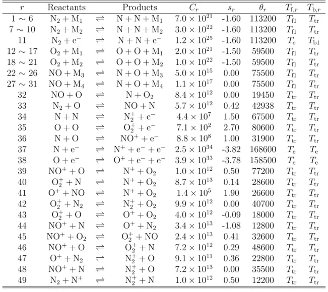
For chemical reactions in high-temperature air, the test gas was assumed to consist of 11 chemical species (N₂, O₂, NO, N⁺₂, O₂⁺, NO⁺, N, O, N⁺, O⁺ and e⁻) and the following 49 reactions are assumed to occur (see Table 2.1).

(24)

1) Heavy-particle impact dissociation,

N₂+M ⇀↽N + N +M (2.35)

O₂+M ⇀↽O + O +M (2.36)

NO +M ⇀↽N + O +M (2.37)

M = N₂,O₂,NO,N⁺₂,O⁺₂,NO⁺,N,O,N⁺,O⁺ 2) Electron impact dissociation,

N₂+ e⁻ ⇀↽ N + N + e⁻ (2.38)

3) NO exchange reaction,

NO + O⇀↽N + O₂ (2.39)

N2+ O⇀↽NO + N (2.40)

4) Associative ionization,

N + N⇀↽N⁺₂ + e⁻ (2.41)

O + O⇀↽O⁺₂ + e⁻ (2.42)

N + O⇀↽NO⁺+ e⁻ (2.43)

5) Electron impact ionization,

N + e⁻⇀↽N⁺+ e⁻+ e⁻ (2.44)

O + e⁻⇀↽O⁺+ e⁻+ e⁻ (2.45)

6) Charge exchange reaction,

NO⁺+ O⇀↽N⁺+ O2 (2.46)

O⁺₂ + N⇀↽N⁺+ O₂ (2.47)

O⁺+ NO⇀↽N⁺+ O₂ (2.48)

O⁺₂ + N₂ ⇀↽N⁺₂ + O₂ (2.49)

O⁺₂ + O⇀↽O⁺+ O₂ (2.50)

NO⁺+ N⇀↽O⁺+ N₂ (2.51)

NO⁺+ O2 ⇀↽O⁺₂ + NO (2.52)

NO⁺+ O⇀↽O⁺₂ + N (2.53)

O⁺+ N₂ ⇀↽N⁺₂ + O (2.54)

NO⁺+ N⇀↽N⁺₂ + O (2.55)

N₂+ N⁺⇀↽N⁺₂ + N (2.56)

The chemical reaction rate was determined with an Arrhenius type form as

k_f,r(T_f,r) =C_rT_f,r^s^rexp(−θ_r/T_f,r). (2.57)

再突入機体周りのプラズマ流れと通信途絶に関する 数値解析的研究