有限温度での中間子遮蔽質量と極質量に対する有効 模型

Kyushu University Institutional Repository

有限温度での中間子遮蔽質量と極質量に対する有効 模型

石井, 優大

https://doi.org/10.15017/1806807

出版情報：Kyushu University, 2016, 博士（理学）, 課程博士 バージョン：

権利関係：Fulltext available.

Effective model for meson screening and pole masses at finite temperature

Masahiro Ishii

Theoretical Nuclear Physics, Department of Physics

Graduate School of Science, Kyushu University

744, Motooka, Nishi-ku, Fukuoka 819-0395, Japan

Abstract

Temperature (T ) dependence of meson mass is an essential quantity char- acterizing properties of hot-QCD matter. T dependence of meson masses is obtainable through measurements of mesons and leptons emitted in heavy- ion collisions, but the experimental results have large uncertainty because of indirect measurements. In this thesis, the meson mass is referred to as

“meson pole mass” in order to distinguish it from “meson screening mass”.

Meson pole and screening masses, M

(T ) and M

(T ), of ξ-meson are defined by the inverse of the exponential decay of the mesonic correlation functions in its temporal and spatial directions, respectively. This definition means that M

(T ) is experimentally measurable, but M

(T ) is not. In lattice QCD (LQCD) simulations at finite T as the first-principle calculation of QCD, the M

(T ) is usually calculated instead of M

(T ), since the tem- poral (imaginary-time) size is limited up to 1/T , but the spatial lattice size doesn’t have such limitation in general. The relation between M

(T ) and M

(T ) at finite T is not understood at all, although M

(0) = M

(0) from the definition.

This thesis aims at predicting meson pole masses M

(T ) reliably from the corresponding meson screening masses M

(T ) calculated with LQCD simulations. For this purpose, we construct the practical and reliable effec- tive model that reproduces LQCD data on M

(T ) and describe the chiral- symmetry restoration and the effective U(1)

-symmetry restoration simulta- neously. In effective models, screening-mass calculations were quite difficult compared with pole-mass calculations, because it required time-consuming numerical calculations. This difficulty is solved by proposing a new method based on the Pauli-Villars regularization and a new prescription in calcu- lating the spatial correlation function for M

(T ). We have then predicted M

(T ) from LQCD data on M

(T ) by using the proposed model for both scalar mesons (ξ = a

, κ, σ and f

) and pseudoscalar ones (ξ = π, K, η and η

). Particularly for η

meson, we have found that the predicted value is consistent with the experimental value recently measured in heavy-ion colli- sions. The model also proposes the following approximate relations between M

(T ) and M

(T ): (i) M

(T ) − M

(T ) ≈ M

(T ) − M

(T ) and (ii) M

(T )/M

(T ) ≈ M

(T )/M

(T ), when ξ

-meson has the same spin-parity as ξ-meson. Using relations (i) and (ii), we can easily estimate M

(T ) from M

(T ), M

(T ) and M

(T ). When ξ

-meson is heavy, M

(T ) may be obtainable with state-of-arts LQCD simulations.

i

Contents

Abstract i

1 Introduction 1

1.1 Quark matter at finite temperature . . . . 1

1.1.1 Deconfinement transition and center symmetry . . . . 2

1.1.2 Spontaneous breaking of chiral symmetry . . . . 4

1.1.3 Instantons and U(1)

symmetry breaking . . . . 5

1.2 Experimental surveys for quark matter . . . . 6

1.3 Lattice QCD and effective models . . . . 6

1.4 Meson masses . . . . 8

1.5 Purpose . . . . 9

2 Formulation for meson screening mass 10 2.1 2-flavor PNJL and EPNJL models . . . 10

2.2 Mesonic correlation functions . . . 12

2.3 Difficulty of screening-mass calculations . . . 15

2.4 Meson screening mass in EPNJL model . . . 16

2.5 Numerical Results . . . 18

2.6 Short Summary . . . 20

3 U (1)

symmetry restoration 22 3.1 U (1)

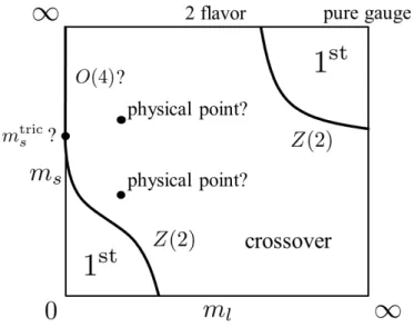
symmetry and Columbia plot . . . 22

3.2 Model setting . . . 24

3.2.1 EPNJL model . . . 24

3.2.2 Mesonic correlation functions . . . 26

3.2.3 Meson pole mass . . . 29

3.2.4 Meson screening mass . . . 29

3.2.5 Meson susceptibility . . . 30

3.3 Numerical Results . . . 31

3.3.1 Meson screening masses . . . 31

3.3.2 Meson susceptibilities . . . 36

3.3.3 The order of chiral transition near the physical point . 38 3.4 Short Summary . . . 40

ii

CONTENTS iii 4 Model prediction for meson pole masses 41

4.1 Formalism . . . 41

4.1.1 Model setting . . . 41

4.1.2 Meson pole masses . . . 45

4.1.3 Meson screening masses . . . 49

4.1.4 Model tuning for LQCD-data analyses . . . 51

4.2 Numerical Results . . . 53

4.2.1 Parameter fitting . . . 53

4.2.2 Meson screening masses . . . 55

4.2.3 Meson pole masses . . . 56

4.2.4 Relation between pole and screening masses . . . 58

4.2.5 Discussion . . . 61

4.3 Short Summary . . . 62

5 Summary and Outlook 64

List of Figures

1.1 Running coupling constant α

as a function of energy scale Q taken from Ref. [1]. . . . 2 2.1 Singularities of χ

(0, q ˜

) in the complex-˜ q plane . . . 16 2.2 T dependence of chiral condensate and Polyakov loop in the

2-flavor system. . . 19 2.3 T dependence of pion and sigma-meson screening masses cal-

culated with the PNJL and EPNJL models. . . 20 3.1 Columbia plot . . . 23 3.2 T dependence of pion and a

-meson screening masses calcu-

lated by EPNJL model with K (T ). . . 31 3.3 T dependence of pion and a

-meson screening masses calcu-

lated by PNJL model with K(T ). . . 32 3.4 T dependence of ∆

and Φ. . . . 33 3.5 T dependence of pion and a

-meson screening masses calcu-

lated by PNJL model with K(0). . . 34 3.6 T dependence of pion and a

-meson screening masses calcu-

lated by PNJL model with K(0). . . 35 3.7 Mass difference ∆M

(T ) between pion and a

-meson screen-

ing masses. . . 35 3.8 T dependence of the difference ∆

between π and a

meson

susceptibilities for two cases of M

(0) = 135 and 200 MeV. . . 36 3.9 T dependence of ∆

and ∆

for M

(0) = 135 MeV. . . 37 3.10 T dependence of ∆

and ∆

for M

(0) = 200 MeV. . . 37 3.11 T dependence of (a) chiral susceptibility χ

and (b) Polyakov-

loop susceptibility ¯ χ

at S-point, P-point and C

-point. . . . 38 3.12 Order of chiral transition near physical point in the m

–m

plane. . . 39 4.1 T dependence of (a) ∆

and (b) ∆M

. . . 53 4.2 T dependence of meson screening masses for (a) pseudoscalar

mesons π, K, η

and (b) scalar mesons a

, κ, σ

. . . 54

iv

LIST OF FIGURES v 4.3 T dependence of meson screening masses for (a) pseudoscalar

mesons π, K, η, η

and (b) scalar mesons a

, κ, σ, f

calculated with the realistic parameter set (A). . . 56 4.4 Model prediction on T dependence of meson pole masses for

(a) pseudoscalar mesons π, K, η, η

and (b) scalar mesons a

, κ, σ, f

57 4.5 Difference between screening and pole masses for (a) pseu-

doscalar mesons π, K, η, η

and (b) scalar mesons a

, κ, σ, f

. . 58 4.6 T dependence of M

/M

and M

/M

for (a) pseu-

doscalar mesons (ξ = K, η, η

, ξ

= π) and (b) scalar mesons (ξ = κ, σ, f

, ξ

= a

). . . 60 4.7 T dependence of channel-mixing effects on (a) η- and η

-meson

screening masses and (b) σ- and f

-meson screening masses. . 61

List of Tables

1.1 Experimental values on current quark masses . . . . 2 2.1 Parameter set of Polyakov-loop potential U . . . 11 2.2 Parameter sets of EPNJL model for 2-flavor and 2+1-flavor

systems. . . . 12 4.1 Model parameters in coupling strengths G

(T ) and G

(T ). . 42 4.2 Two model-parameter sets . . . 44 4.3 Physical quantities at vacuum calculated with the parameter

set (A) of Table 4.2 and the corresponding experimental or empirical values. . . . 45

vi

Chapter 1 Introduction

1.1 Quark matter at finite temperature

Strong interaction is one of the four basic interactions existing in the nature.

The interaction is working among quarks and gluons. In this sense, quarks and gluons are fundamental particles in the nature. At low temperature (T ), they are confined into hadrons by strong interaction. As T increases, the mean distance among hadrons and anti-hadrons gets shorter, and con- sequently hadrons and anti-hadrons start to overlap with each other. At extremely high T , hadrons are considered to melt into quarks and gluons gas, i.e., quark–gluon plasma (QGP). In fact, the QGP phase exists in the early universe, and the QGP phase is changed into the hadron phase as a result of the cooling (expansion) of the universe. The transition between the hadron and QGP phases has been studied experimentally and theoretically;

however, it has not been revealed yet. Elucidation of quark and hadron mat- ters at finite T is an essential subject between particle physics and cosmology, that is, a bridge between the two fields.

The strong interaction is known to be described by quantum chromody- namics (QCD). The Lagrangian density in Euclid spacetime is

L

= ¯ ψ (γ

D

+ ˆ m) ψ + 1 2 tr

! F

"

(1.1) for quark fields ψ and gluon fields A

. The trace tr

is taken in color space.

The ψ is ψ = (ψ

, ψ

, ψ

, ψ

, ψ

, ψ

)

for up (u), down (d), strange (s), charm (c), bottom (b), and top (t) quarks. The A

are connected with ψ through the covariant derivative D

= ∂

− igA

with the coupling constant g. Gluon dynamics is organized by the field strength tensor F

:

F

= ∂

A

− ∂

A

+ ig[A

, A

]. (1.2) The current-quark-mass matrix ˆ m is ˆ m = diag(m

, m

, m

, m

, m

, m

) and the values are tabulated in Table 1.1. In this study, we focus on the nonper- turbative aspects of hot-QCD matter that are realized in lower temperatures of order Λ

∼ 200 MeV as a typical energy scale of QCD. Therefore we consider dynamics of the light quarks (u, d, and s quarks) whose current masses are smaller than Λ

.

1

Table 1.1: Experimental values on current quark masses taken from Ref. [1].

m

m

m

m

m

m

2.3 MeV 4.8 MeV 95 MeV 1.275 GeV 4.18 GeV 160 GeV

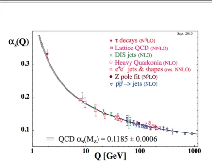
Fig. 1.1: Running coupling constant α

as a function of energy scale Q taken from Ref. [1].

The most important property of QCD is asymptotic freedom. Strong in- teraction among quarks and gluons gets weaker as the energy scale Q goes up. The Q dependence of the running coupling constant α

(Q) is experimen- tally measured in the deep-inelastic scattering (DIS) between leptons and hadrons, τ decay, and so on, as shown in Fig. 1.1. The symbols denote the experimental results and the lines denote the theoretical predictions based on perturbation theory. The perturbation well reproduces the experimental results in Q > 1 GeV.

In low Q ≤ 1 GeV, the QCD vacuum has nonperturbative structures such as color confinement, the spontaneous breaking of chiral symmetry, and the existence of instantons and antiinstantons. They come from large/local gauge and global symmetries that the QCD Lagrangian possesses.

1.1.1 Deconfinement transition and center symmetry

The transition from the hadron (confinement) phase at low T to the QGP

(deconfinement) phase at high T is characterized by the spontaneous breaking

of “center symmetry”, as shown below. The symmetry is exact in the pure

Yang–Mills theory, but not in QCD. The pure Yang–Mills theory corresponds

to QCD in the limit of heavy quark mass. In QCD, the expectation value

1.1. QUARK MATTER AT FINITE TEMPERATURE 3

⟨ O ⟩ of an operator O is obtained with the path integral as

⟨ O ⟩ = 1 Z

#

BC

D ψ D ψ ¯ D A

O[ψ, ψ, A ¯

] exp $

− (S

[ψ, ψ, A ¯

] + S

[A

]) % , (1.3) where the quark and Yang–Mills parts of QCD action, S

and S

, are

S

=

#

dτ

#

d

x ψ(γ ¯

D

+ ˆ m)ψ, S

=

#

dτ

#

d

x 1

2 tr

(F

) (1.4) in Euclidean spacetime (x

) = (τ, x) where imaginary time τ has an upper limit β = 1/T . The partition function Z of QCD is described as

Z =

#

BC

D ψ D ψ ¯ D A

exp $

− (S

[ψ, ψ, A ¯

] + S

[A

]) %

. (1.5)

The subscript “BC” of the integral means the boundary conditions

ψ (τ + β, x) = − ψ (τ, x) , ψ ¯ (τ + β, x) = − ψ ¯ (τ, x) , (1.6) A

(τ + β, x) = A

(τ, x) (1.7) for ψ, ψ ¯ and A

. In the τ direction, we should impose the antiperiodic bound- ary condition on fermions such as quarks, and the periodic boundary condi- tion on bosons such as gluons. Now we consider the following local SU(3)

gauge transformation

ψ(x) → ψ

(x) = V (x)ψ(x), A

(x) → A

(x) = V (x)

&

A

(x) − i g ∂

'

V

(x) (1.8) with the aperiodic boundary condition

V (τ + β, x) = zV (τ, x) (1.9)

for V (x) in the τ direction. The symbol z is the “center” of SU(3)

group that commutes with all the elements of SU(3)

, and it is defined as

z = e

I

≡ z

I

(k = 0, 1, 2) (1.10) with the unit matrix I

in color space. We call the transformation as “Z

transformation” in order to distinguish it from the usual gauge transforma- tion (1.8)-(1.9) with z replaced by I

. In QCD, the Lagrangian is invariant under the Z

transformation. This symmetry is then referred to be “center symmetry”. However, the Z

transformation modifies the boundary condi- tion for ψ, ψ ¯ as

ψ

(τ + β, x) = − z

ψ

(τ, x) , ψ ¯

(τ + β, x) = − z

ψ ¯

(τ, x) . (1.11)

Therefore, center symmetry is explicitly broken through the boundary condi-

tion for dynamical quarks, although it is preserved in QCD Lagrangian itself.

Center symmetry becomes exact in pure Yang–Mills theory, since the theory has no quark-dynamics.

Center symmetry is considered to be approximately good in QCD, partic- ularly for heavy quarks. An order parameter of the center-symmetry breaking is the Polyakov loop Φ ≡ ⟨ Φ(x) ⟩ where the Polyakov-loop operator Φ(x) is defined by

Φ(x) = 1

3 tr

T exp

&

ig

#

dτ A

(τ, x) '

. (1.12)

Here, the symbol T stands for the path ordering for τ . Under the Z

trans- formation, the Polyakov-loop operator is transformed as

Φ(x) → Φ

(x) = z

Φ(x). (1.13) This property means that Φ = 0 corresponds to the center-symmetric phase and Φ ̸ = 0 does to the center-symmetry broken phase. The Polyakov loop is related to an excitation energy F

of single heavy quark as [2]

Φ ∝ exp ( − βF

). (1.14)

In the confinement phase, F

should be infinity, so that Φ = 0. Therefore, the confinement phase is center-symmetric. In the deconfinement phase, F

is finite, so that Φ ̸ = 0. Hence, center symmetry is broken in the deconfinement phase. The Polyakov loop is thus an order parameter of the breaking of center symmetry, that is, the confinement/deconfinement transition:

Φ =

( 0 for the confinement phase with center symmetry, finite for the deconfinement phase without center symmetry.

(1.15)

1.1.2 Spontaneous breaking of chiral symmetry

In the chiral limit of m

= m

= m

= 0, QCD Lagrangian (1.1) is invariant under the flavor U(3)

× U (3)

rotation for the right- and left-handed quarks, ψ

and ψ

, defined by

ψ

= P

ψ, ψ

= P

ψ (1.16)

with ψ = (ψ

, ψ

, ψ

)

and the projection operators P

= (1 ± γ

)/2. We rewrite the Lagrangian with ψ

and ψ

fields as

L

= ¯ ψ

γ

D

ψ

+ ¯ ψ

γ

D

ψ

+ ( ¯ ψ

mψ ˆ

+ ¯ ψ

mψ ˆ

) + · · · , (1.17) where ˆ m = diag(m

, m

, m

). The global U(3)

× U (3)

transformation with rotation angles α and β is

ψ

→ ψ

= U (α)ψ

, ψ

→ ψ

= U (β)ψ

,

ψ ¯

→ ψ ¯

= ¯ ψ

U

(α), ψ ¯

→ ψ ¯

= ¯ ψ

U

(β). (1.18)

1.1. QUARK MATTER AT FINITE TEMPERATURE 5 Here, U (θ) is a unitary matrix with rotation angles θ = (θ

, ..., θ

):

U (θ) = exp )

i

*

θ

T

+

(1.19) with the matrices T

defined by

T

= , 2

3 I

, T

= λ

2 (a = 1, 2, ..., 8), (1.20) where the I

is the unit matrix and the λ

correspond to the Gell-Mann matrices in flavor space. The transformation (1.18) with β = − α is called

“chiral transformation”, and QCD Lagrangian (1.17) is invariant under the chiral transformation in the chiral limit. If one considers finite current- quark masses, chiral symmetry is explicitly broken by the mass terms in QCD Lagrangian (1.17). The explicit breaking seems to be small, since m

, m

, m

< Λ

∼ 200 MeV. Therefore chiral symmetry is approximately good in QCD Lagrangian. However, in QCD vacuum, chiral symmetry is not preserved and U (3)

× U (3)

symmetry is broken into SU (3)

× U (1)

× U (1)

symmetry. This is called “the spontaneous breaking of chiral symmetry”. An order parameter of the breaking is chiral condensate

⟨ ψ ¯

ψ

⟩ = ⟨ ψ ¯

ψ

⟩ + ⟨ ψ ¯

ψ

⟩ (1.21) for flavor f . The condition ⟨ ψ ¯

ψ

⟩ = 0 corresponds to the chiral-symmetric phase and ⟨ ψ ¯

ψ

⟩ ̸ = 0 does to the chiral-symmetry broken phase as

⟨ ψ ¯

ψ

⟩ =

( 0 for the chiral-symmetric phase,

finite for the chiral-symmetry broken phase. (1.22)

1.1.3 Instantons and U (1)

symmetry breaking

In Ref. [3], Weinberg considered the relation between pion mass (M

) and η

-meson mass (M

). He pointed out that current algebra indicates M

≤

√ 3M

and this result is inconsistent with the experimental result M

≫

√ 3M

. This problem was solved by considering quantum anomaly of axial current and introducing topologically nontrivial gauge configurations, each with different winding number ν, in QCD vacuum. In the chiral limit ( ˆ m = 0), the quantum anomaly leads to

∂

j

(x) = − 2N

Q(x) (1.23) as a relation between the U(1)

current j

(x) and the topological charge density Q(x), which are defined by

j

(x) = ¯ ψ(x)γ

γ

ψ(x), Q(x) = g

16π

tr

-

F

(x) ˜ F

(x) .

(1.24)

with the number N

of flavors and F ˜

(x) = 1

2 ϵ

F

(x). (1.25) The winding number ν is defined by

ν ≡

#

d

x Q(x). (1.26)

The nontrivial gauge configuration with ν = 1 (ν = − 1) is called instanton (antiinstanton).

In the operator level, U (1)

symmetry is always broken through Q(x), as shown in Eq. (1.23). For the expectation value of Eq. (1.23), the U (1)

- symmetry breaking is affected by the nontrivial structure of QCD vacuum.

After integrating both the sides of Eq. (1.23) in spacetime x, global U (1)

symmetry is approximately conserved if QCD vacuum is dominated by topo- logically trivial (ν = 0) gauge configurations [4]. In this sense, the U (1)

- symmetry breaking due to finite ν is simply called “U (1)

anomaly” in this thesis.

1.2 Experimental surveys for quark matter

In experiments, properties of hot-QCD matter have been explored through measurements of hadrons and leptons produced in heavy-ion collisions. Heavy ions are collided with incident energies large enough to create QGP. In Rel- ativistic heavy-ion collider (RHIC) experiments [5], QGP is considered to be realized in the intermediate stage of the collisions by measuring various kinds of flows and jets of hadrons. Similar measurements have been performed by changing incident energies, centrality, and targets with Large Hadron Col- lider (LHC) in CERN, Facility for Antiproton and Ion Research (FAIR) in GSI, Nuclotron-based Ion Collider fAcility (NICA) in Dubna, and Japan Proton Accelerator Research Complex (JPARC) in KEK.

T dependence of meson mass is the essential quantity that characterizes properties of hot-QCD matter. In principle, one can determine T dependence of meson masses through measurements of mesons emitted in heavy-ion col- lisions. However, the experimental results have large uncertainty in general, because they are indirect measurements. In fact, η

-meson mass measured at finite T has large errors that mainly come from data analyses [6].

1.3 Lattice QCD and effective models

Lattice QCD (LQCD) simulation is the first-principle calculation of QCD and hot-QCD. In the simulations, spacetime x is discretized into a lattice.

Each lattice point is labeled by a vector n = (n

, n

, n

, n

), where x

= n

a

1.3. LATTICE QCD AND EFFECTIVE MODELS 7 for lattice spacing a and integer n

. Quark fields ψ(x) and ¯ ψ(x) are defined on each lattice point. For convenience, we introduce dimensionless quark fields ψ

and ¯ ψ

on each lattice point:

ψ(x) = a

ψ

, ψ(x) = ¯ a

ψ ¯

. (1.27) The factor a

is necessary to make ψ

and ¯ ψ

dimensionless. Gluon fields A

(x) are described as link variables

U

≡ U (na, na + ˆ µa) (1.28) with the comparator

U (x, y ) ≡ P exp /

ig

#

dz

A

(z) 0

, (1.29)

where ˆ µ is the unit vector in the µ direction and the symbol P is the path or- dering for the z-direction. The QCD partition function Z is then represented by

Z =

#

D ψ D ψ ¯ D U exp $

− !

S

[ψ, ψ, U ¯ ] + S

[U ] "%

=

#

D U det M [U] exp [ − S

[U ]], (1.30) where see for example Ref. [7] for the explicit forms of S

, S

, M and the path integral. The path integral is numerically performed by using Monte- Carlo method with the importance sampling. When det M [U ] is complex, the importance sampling breaks down. This problem is called “Sign problem”.

This problem occurs for finite quark-number chemical potential µ

. For this reason, LQCD simulations provide a lot of results particularly at µ

= 0.

As an approach complementary to LQCD simulations, properties of QCD and hot-QCD have been studied intensively by effective models such as the Nambu–Jona-Lasinio (NJL) model and the Polyakov-loop extended Nambu–

Jona-Lasinio (PNJL) model [8–24]. In the NJL model, U (1)

anomaly and

the spontaneous breaking of chiral symmetry are taken into account. In the

PNJL model, confinement is approximately considered through the Polyakov

loop Φ, in addition to U (1)

anomaly and the spontaneous breaking of chiral

symmetry. These models have been applied for many phenomena. In partic-

ular, the PNJL model has been used to investigate the relation between the

chiral and the deconfinement transitions. Lately, a Polyakov-loop (Φ) depen-

dent four-quark interaction was introduced so as to enhance the correlation

between the two transitions [25,26]. The PNJL model with the entanglement

(Φ-dependent) four-quark interaction is now called the entanglement-PNJL

(EPNJL) model [25, 26]. The EPNJL model is successful in reproducing

LQCD results in the imaginary µ

region [27, 28] and the real isospin chemi-

cal potential region [29] where LQCD is free from the Sign problem.

1.4 Meson masses

Meson mass is a key characterizing QCD vacuum. T dependence of me- son masses plays an important role in understanding properties of hot-QCD matter, for example, in determining reaction rates of hadron-hadron colli- sions and dilepton production.

In this thesis, the meson mass is referred to as “meson pole mass” in order to distinguish it from “meson screening mass”. Meson pole and screen- ing masses, M

(T ) and M

(T ), of ξ-meson are defined by the inverse of the exponential decay of the mesonic correlation functions in its temporal τ- and spatial x-directions, respectively. Obviously, this definition shows that M

(T ) is experimentally measurable, but M

(T ) is not. On the other hand, in LQCD simulations at finite T as the first-principle calculation of QCD, the M

(T ) is usually calculated instead of M

(T ), since the tem- poral (imaginary-time) size is limited up to 1/T , but the spatial lattice size doesn’t have such limitation in general. The relation between M

(T ) and M

(T ) at finite T is not understood at all, although M

(0) = M

(0) from the definition. T dependence of light-meson screening masses was evalu- ated lately in a wide range of 140 < ∼ T < ∼ 800 MeV by using 2+1-flavor LQCD simulations with improved (p4) staggered fermions [30]. Thus, the M

(T ) are available with LQCD simulations, but not measurable experimentally.

The M

(T ) are thus obtainable with LQCD simulations but not with experiments. In contrast, the M

(T ) are experimentally measurable but hard to obtain with LQCD simulations. If we can predict M

(T ) theoreti- cally from LQCD results on M

(T ), we can compare the predicted M

(T ) with the corresponding experimental data directly. Furthermore, when ex- perimental data are not available for M

(T ) of interest, such a prediction may be useful in experimental analyses.

As a complementary approach to LQCD simulations for M

(T ) and experimental measurements for M

(T ), we can consider effective models such as the PNJL model [8–24] and the EPNJL model [25,26]. T dependence of M

(T ) was often studied with the NJL-type effective models [8, 12, 19, 23,24,31]. These models well describe M

(T ) at T = 0, but it was difficult to calculate M

(T ) at finite T with the NJL-type models. However, this problem was solved very recently; see Chapter 2 for the detail.

Throughout these discussions, we can find the following three problems in order to obtain M

(T ) accurately:

(I) In principle, T dependence of M

(T ) can be determined from mea- surements in heavy-ion collisions. However, the measurements are in- direct, so that the experimental results have large uncertainty.

(II) LQCD simulation is the first-principle calculation of QCD. However,

the calculation of M

(T ) is quite difficult compared with M

(T ),

1.5. PURPOSE 9 because the imaginary-time size is limited up to 1/T . The difficulty becomes more serious as T increases.

(III) In effective models, screening-mass calculations were quite difficult compared with pole-mass calculations.

1.5 Purpose

The aim of this thesis is to make a reliable model prediction on M

(T ) from the corresponding M

(T ) calculated with LQCD simulations. We solve problems (I) ∼ (III) to accomplish the aim.

In Chapter 2, we solve problem (III) by considering the following two prescriptions: (1) The Pauli-Villars regularization and (2) a new prescrip- tion in calculating the spatial correlation function for M

(T ). These two prescriptions extremely reduce numerical costs, as shown in Chapter 2.

In Chapter 3, we solve problems (I) and (II) particularly for π and a

mesons by proposing a new version of EPNJL model that reproduces LQCD data on M

(T ) and M

(T ).

In Chapter 4, we solve problems (I) and (II) generally for scalar and pseu- doscalar mesons by proposing a new version of PNJL model that reproduces LQCD data on M

(T ) for ξ = π, K, η

, a

, κ, σ

mesons.

This thesis is based on the following two published and one submitted papers:

• Effective model approach to meson screening masses at finite tempera- ture, M. Ishii, T. Sasaki, K. Kashiwa, H. Kouno, and M. Yahiro, Phys.

Rev. D 89, 071901(R) (2014).

• Determination of U (1)

restoration from pion and a

-meson screening masses: Toward the chiral regime, M. Ishii, K. Yonemura, J. Takahashi, H. Kouno, and M. Yahiro, Phys. Rev. D 93, 016002 (2016).

• Model prediction for temperature dependence of meson pole masses from lattice QCD results on meson screening masses, M. Ishii, H.

Kouno, and M. Yahiro, submitted in Physical Review D.

Chapter 2

Formulation for meson screening mass

In this chapter, we evaluate temperature (T ) dependence of pion and sigma- meson screening masses by using the Polyakov-loop extended Nambu–Jona- Lasinio (PNJL) model and the entanglement-PNJL (EPNJL) model. For this purpose, we propose a practical method of calculating meson screen- ing masses in NJL-type effective models. Our method solves the well-known problem that the evaluation of screening masses is difficult in NJL-type ef- fective models. The method is based on the Pauli–Villars (PV) regulariza- tion and a new prescription of calculating the correlation function for meson screening mass. We first show that the EPNJL model with the PV reg- ularization is successful in reproducing 2-flavor lattice QCD results on T dependence of the chiral condensate and the Polyakov loop. We then ap- ply the method to recent 2+1-flavor lattice QCD results on T dependence of pion screening mass. Since pion is composed of u and d quarks, we use 2-flavor EPNJL model for simplicity. This approximation is good enough for qualitative discussion.

2.1 2-flavor PNJL and EPNJL models

The PNJL model is one of effective models for QCD in the low-energy region.

The model describes the spontaneous breaking of chiral symmetry and color confinement of quarks at the same time. The Lagrangian density of 2-flavor PNJL model in Minkowski space is defined as

L

= ¯ ψ(iγ

D

− m ˆ

)ψ + G

[( ¯ ψψ)

+ ( ¯ ψiγ

τ ψ)

] − U (Φ[A], Φ[A], T ¯ ) (2.1) with the u-, d-quark fields ψ = (ψ

, ψ

)

, the current-quark-mass matrix

ˆ

m

= diag(m

, m

) and the Pauli matrices τ = (τ

, τ

, τ

) in isospin space.

We consider the isospin-symmetric case for simplicity: m

= m

= m

. The gauge fields A

are introduced through the covariant derivative

D

= ∂

+ iA

, (2.2)

10

2.1. 2-FLAVOR PNJL AND EPNJL MODELS 11 where the A

are assumed to be static background fields and A

= gδ

A

=

− igδ

A

for the coupling constant g. The Polyakov loop Φ and its conjugate Φ ¯ are then obtained in the Polyakov gauge by

Φ = 1

3 tr

(L), Φ ¯ = 1

3 tr

(L

) (2.3)

with L = exp[iA

/T ] = exp[idiag(A

, A

, A

)/T ] for the classical variables A

satisfying that A

+ A

+ A

= 0.

The A

are not uniquely determined from Φ and ¯ Φ, because of the gauge symmetry, e.g., Φ and ¯ Φ are invariant under the interchange of A

, A

and A

. The arbitrariness does not change any physics. Particularly for zero quark chemical potential (µ = 0), Φ equals to ¯ Φ, because the QCD La- grangian (1.1) is invariant under the charge conjugation. Hence it is possible to determine A

, A

and A

as

A

= − A

= cos

&

3Φ − 1 2

'

T, A

= 0 (2.4) for µ = 0. Here, Φ and ¯ Φ are mainly governed by the Polyakov-loop potential U in Eq. (2.1). We use the logarithm-type Polyakov-loop potential [18]

U (Φ, Φ, T ¯ ) = T

/

− a(T )

2 Φ Φ ¯ + b(T ) ln 1

1 − 6Φ Φ ¯ + 4(Φ

+ ¯ Φ

) − 3(Φ Φ) ¯

2 0 , (2.5) a(T ) = a

+ a

&

T

T

' + a

&

T

T

'

, b(T ) = b

&

T

T

'

. (2.6)

The parameter set in U is fitted to reproduce LQCD data at finite T in the pure gauge limit, i.e., QCD without dynamical quarks. The parameter set is tabulated in Table 2.1. The potential yields the first-order deconfinement Table 2.1: Parameter set of Polyakov-loop potential U . The parameters are taken from Ref. [18].

a

a

a

b

T

(Pure gauge) 3.51 − 2.47 15.2 − 1.75 270 [MeV]

phase transition at T = T

. In the pure gauge limit, LQCD data show the

phase transition at T = 270 MeV. Hence the parameter T

is often set to

270 MeV. However, if one considers dynamical quarks, the PNJL model with

this value of T

yields a larger value of pseudocritical temperature for the

deconfinement transition than the LQCD prediction. This problem can be

solved by rescaling T

, as shown in Ref. [25]. Therefore, we treat T

as an

adjustable parameter.

The EPNJL model is an extension of the PNJL model. In the EPNJL model, the coupling constant of the four-quark interaction is assumed to depend on Φ and ¯ Φ [25, 26]:

G

(Φ) = G

(0) · $

1 − α

Φ Φ ¯ − α

!

Φ

+ ¯ Φ

"%

. (2.7)

When α

= α

= 0, the EPNJL model is reduced to the PNJL model. The parameters α

, α

and T

in the EPNJL model are determined to reproduce LQCD data on the chiral-transition temperature T

. The parameters are tabulated in Table 2.2. When we analyze 2-flavor LQCD results on T depen- dence of chiral condensate and Polyakov loop, we use the first parameter set named “2-flavor” in Table 2.2. When we analyze 2+1-flavor LQCD results on T dependence of pion screening mass, we use second parameter set named

“2+1-flavor” in Table 2.2; see Sec. 2.5 for the detail.

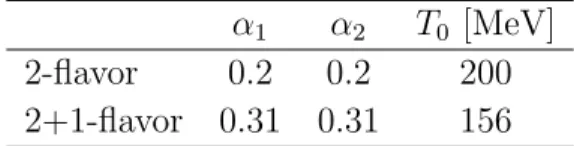
Table 2.2: Parameter sets of EPNJL model for 2-flavor and 2+1-flavor sys- tems.

α

α

T

[MeV]

2-flavor 0.2 0.2 200 2+1-flavor 0.31 0.31 156

2.2 Mesonic correlation functions

We derive the equations for pion and sigma-meson screening masses. First, we determine the dressed quark propagator by using the mean-field (Hartree) approximation. We then treat a meson propagation as a mesonic fluctuation from the mean-field variable by taking the random-phase approximation.

Making the mean-field approximation to the Lagrangian density (2.1) leads to the linearized Lagrangian density

L

= ¯ ψS

ψ − U

(σ, Φ, Φ) ¯ − U (Φ[A], Φ[A], T ¯ ), (2.8) where S is the dressed quark propagator

S = 1

iγ

∂

− iγ

A

− M ˆ (2.9)

with the effective-quark-mass matrix ˆ M = diag(M, M ) satisfying M = m

−

2G

(Φ)σ and the mesonic potential U

= G

(Φ)σ

. The variable σ means

the chiral condensate: σ = ⟨ ψψ ¯ ⟩ . Making the path integral over the quark

2.2. MESONIC CORRELATION FUNCTIONS 13 field, one can get the thermodynamic potential (per unit volume) as

Ω

(σ, Φ, Φ, T ¯ ) = U

+ U − 2N

# d

p (2π)

3 3E

+ 1

β ln [1 + 3(Φ + ¯ Φe

)e

+ e

] + 1

β ln [1 + 3( ¯ Φ + Φe

)e

+ e

] 4

(2.10) with β = 1/T , E

= 5

p

+ M

and the number N

of flavors. Mean-field variables (σ, Φ and ¯ Φ) are determined to minimize Ω

.

The mesonic current corresponding to ξ = π or σ meson is

J

(x) = ¯ ψ(x)Γ

ψ(x) − ⟨ ψ(x)Γ ¯

ψ(x) ⟩ , (2.11) where the matrix Γ

has the color, flavor and Dirac indices. The matrix Γ

is Γ

= I

⊗ I

⊗ I

for ξ = σ and Γ

= I

⊗ iγ

⊗ τ

for ξ = π, where I

, I

and I

are the unit matrices in color, Dirac and flavor spaces, respectively.

The mesonic correlation function ζ

(t, x) in coordinate space x = (t, x) is defined by

ζ

(t, x) ≡ ⟨ 0 | T -

J

(x)J

(0) .

| 0 ⟩ , (2.12)

where the symbol T stands for the time-ordered product. The mesonic cor- relation function χ

(q

, q

) in momentum space q = (q

, q) is obtained as the Fourier transformation of ζ

(t, x):

χ

(q

, q

) = i

#

d

x e

ζ

(t, x). (2.13) Using the random-phase (ring) approximation, one can obtain the Schwinger- Dyson equation  

χ

(q

, q

) = Π

(q

, q

) + 2G

(Φ)Π

(q

, q

)χ

(q

, q

) (2.14) for χ

(q

, q

), where the one-loop polarization function Π

(q

, q

) is defined as

Π

(q

, q

) ≡ ( − i)

# d

p

(2π)

tr

(Γ

iS(p

+ q)Γ

iS(p

)) (2.15) with p

= (p

+ iA

, p) and the dressed quark propagator S(p) in the Hartree approximation. The trace tr

is taken in color, flavor and Dirac spaces.

The solution to Eq. (2.14) is

χ

= Π

1 − 2G

(Φ)Π

. (2.16)

The Π

are explicitly obtained by Π

= i

# d

p

(2π)

Tr 3 { γ

(p

+ q)

+ M } (γ

p

+ M ) { (p

+ q)

− M

} (p

− M

)

4

= 2iN

[I

+ I

− (q

− 4M

)I

], (2.17) Π

= i

# d

p (2π)

Tr 3

(iγ

τ

) { γ

(p

+ q)

+ M }

{ (p

+ q)

− M

} × (iγ

τ

) (γ

p

+ M ) (p

− M

)

4

= 2iN

[I

+ I

− q

I

], (2.18)

with

I

=

# d

p (2π)

tr

3 1

p

− M

4

, (2.19)

I

=

# d

p (2π)

tr

3 1

(p

+ q)

− M

4 , (2.20)

I

=

# d

p (2π)

tr

3 1

{ (p

+ q)

− M

} (p

− M

) 4 ,

(2.21) where trace tr

means the trace of color matrix. For finite T , the correspond- ing equations are obtained by the replacement

p

→ iω

= i(2n + 1)πT,

# d

p

(2π)

→ iT

*

# d

p

(2π)

. (2.22)

In this thesis, we refer to the summation over n as “Matsubara summation”

and the integral over p as “internal-momentum integration”.

We need to regularize the momentum p integrals in the thermodynamic potential Ω

of Eq. (2.10) and in the three functions I

, I

, I

. Usually, the three-dimensional momentum-cutoff regularization

# d

p (2π)

→

#

|p|≤Λ

d

p

(2π)

(2.23)

is taken in NJL-type effective models, where Λ is a cutoff parameter. How- ever, the regularization breaks Lorentz invariance. In this thesis, we take the Pauli-Villars (PV) regularization [32] that preserves Lorentz invariance.

The original version of PV regularization breaks chiral symmetry explicitly, since the regularization introduces auxiliary particles with heavy masses. In addition, we cannot take their masses infinity, because the present model is nonrenormalizable. This problem is solved by E. Ruiz Arriola and L.L.

Salcedo in Ref. [33].

Here we explain the PV regularization for the thermodynamic potential Ω

and the three functions I

, I

, I

. For convenience, we divide Ω

into Ω

= U

+ U + N

Ω

(M ), and represent I

and I

by I(M ) and

2.3. DIFFICULTY OF SCREENING-MASS CALCULATIONS 15 I

by I

(M ). In the PV scheme, the functions Ω

(M ), I(M ) and I

(M ) are regularized as

Ω

(M) =

*

C

Ω

(M

),

I

(M) =

*

C

I(M

), I

(M) =

*

C

I

(M

), (2.24) where M

= M and the M

(α = 1, 2) mean masses of auxiliary particles.

The parameters M

and C

should satisfy the condition

*

C

= 0,

*

C

M

= 0 (2.25)

to remove the quartic, the quadratic and the logarithmic divergence in I

, I

, I

, and Ω

. We assume (C

, C

, C

) = (1, 1, − 2) and (M

, M

) = (M

+ 2Λ

, M

+ Λ

), following Ref. [34]. We keep the parameter Λ finite even after the subtraction (2.24), since the present model is non-renormalizable.

In the present parameterization, logarithmic divergence partially remains in Ω

(M) even after the subtraction (2.24), but the term does not depend on the mean-field variables (σ, Φ, Φ) and is irrelevant to the determination of ¯ mean-field variables for any T . Therefore we can simply drop the term.

2.3 Difficulty of screening-mass calculations

The NJL-type effective models are very useful. In fact, meson pole masses have been predicted by the models, particularly for light scalar and pseu- doscalar mesons. In contrast, the evaluation of meson screening masses was quite difficult. The difficulty comes from the following two problems. One is that the NJL-type models are nonrenormalizable and thereby the regular- ization is necessary in the model calculations. So far, the three-dimensional momentum-cutoff regularization (2.23) was often taken. However, the regu- larization breaks Lorentz invariance. As a result of this breaking, the spatial correlation function ζ

(0, x) has unphysical oscillations [35]. This makes it quite difficult to determine meson screening mass (M

) from the exponential decay of ζ

(0, x) at large distance (r = | x | ):

M

≡ − lim

r→∞

d ln ζ

(0, x)

dr . (2.26)

Another problem is difficulty of the Fourier transformation ζ

(0, x) =

# d

q

(2π)

χ

(0, q

)e

= 1 4π

ir

#

−∞

d˜ q qχ ˜

(0, q ˜

)e

, (2.27)

where ˜ q = ±| q | . In the model approach, the correlation function χ

(0, q ˜

) is calculated first in momentum space and is Fourier transformed to the func- tion ζ

(0, x) in coordinate space. In the integrand of Eq.(2.27), ˜ qχ

(0, q ˜

) is slowly damping with ˜ q, whereas e

is highly oscillatory particularly at large r where M

is determined. This property makes direct numerical cal- culations difficult. In general, this problem is avoidable with contour integral in complex-˜ q plane. However, the contour integral is still difficult because unphysical cuts are present in the vicinity of the real axis [35]; see the left panel of Fig. 2.1, where the limit of ϵ → 0 should be taken after the Fourier transformation.

Fig. 2.1: Singularities of χ

(0, q ˜

) in the complex-˜ q plane based on the pre- vious formulation [35] (left) and the present formulation (right). The wavy lines denote cuts and the open points represent the branch points of cuts.

The closed points correspond to poles.

2.4 Meson screening mass in EPNJL model

The meson screening mass M

is determined from the exponential damping of ζ

(0, x) that is the Fourier transform of χ

(0, q ˜

), as shown in Eq. (2.27).

In the previous formalism [35], however, heavy numerical calculations are re- quired in the Fourier transform. We first explain the difficulty in the previous formalism [35]. After making the PV regularization and taking Matsubara (n) summation before the p integral in Eq. (2.22), the function I

(0, q ˜

) in χ

(0, q ˜

) contains a term I

= I

+ I

defined by

I

(0, q ˜

) = − iN

16π

*

C

/

ln M

+ f

&

2M

˜ q

'0

, (2.28)

f

(x) = √

1 + x

ln ) √

1 + x

+ 1

√ 1 + x

− 1 +

(2.29)

2.4. MESON SCREENING MASS IN EPNJL MODEL 17 and

I

(0, q ˜

) = iN

16π

*

C

#

0

dp f

(p, q) ˜ !

F

+ F

"

, (2.30)

f

(p, q) = ˜ 1 E

p

˜ q ln

&

(˜ q − 2p)

+ ϵ

(˜ q + 2p)

+ ϵ

'

, (2.31)

where the Fermi distribution functions F

are defined as F

= 1

N

*

j=1

1

exp [β(E

± iA

)] + 1 (2.32) with number N

of colors. In Eq. (2.31), the ϵ

term is added to make the p integral well-defined at ˜ q = ± 2p, but this requires the limit of ϵ → 0 finally.

As shown in the left panel of Fig. 2.1, f

(2M

/˜ q) has the vacuum cuts and f

(p, q) possesses temperature cuts in the complex ˜ ˜ q plane. In the upper- half plane where contour integral is performed, the cuts contribute to the ˜ q integral in addition to the pole at ˜ q = iM

determined by

$ 1 − 2G

(Φ)Π

(0, q ˜

) %66

˜

q=iM_ξ^scr

= 0. (2.33) It is not easy to evaluate the temperature-cut contribution, since in Eq. (2.27) the integrand is slowly damping and highly oscillating with ˜ q near the real axis in the complex ˜ q plane. Furthermore we have to take the limit of ϵ → 0 finally.

The problem mentioned above can be solved by taking the n summation after making the p integral, as shown below. Following this procedure, we get I

(0, q ˜

) as an n-summation of analytic functions:

I

(0, q ˜

) = iT 2π

Nc

*

j=1

*

*

C

#

dx

#

0

d ˜ k k ˜

[˜ k

+ (x − x

)˜ q

+ M

]

= iT 4π q ˜

*

j,n,α

C

sin

-

7

˜ q²

4

+ M

. (2.34)

with

M

(T ) = 7

M

+ { (2n + 1)πT + A

}

. (2.35) We have numerically checked that the convergence of the n summation is quite fast in Eq. (2.34). In the upper-half plane, each term of I

(0, q ˜

) has a cut starting from 2iM

on the imaginary axis. The cut is shown in the right panel of Fig. 2.1. The lowest branch point is

˜

q = iM

≡ 2iM

(2.36)

Hence M

is regarded as “threshold mass”, because that the meson screening-

mass spectrum becomes continuous above the point.

When M

< M

, the pole at ˜ q = iM

is isolated from the cut well.

This means that one can take the contour (A → B → C → D → A) shown in the right panel of Fig. 2.1. The ˜ q integral of ˜ qχ

(0, q ˜

)e

on the real axis in Eq. (2.27) is then obtainable from the residue at the pole and the line integral from point C to point D. The former behaves as exp[ − M

r]/r at large r and the latter as exp [ − M

r]/r. The behavior of ζ

(0, x) at large r = | x | is thus determined by the pole. Therefore, we can evaluate the screening mass from the location of the pole in the complex-˜ q plane without performing the

˜

q integral. In the high-T limit, the threshold mass tends to 2πT . This result is consistent with that of perturbative QCD [36].

2.5 Numerical Results

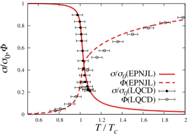
First, we show that the EPNJL model with PV regularization well describes the chiral symmetry restoration. As already mentioned in Sec. 2.2, the orig- inal version of PV regularization breaks chiral symmetry explicitly, since the regularization introduces auxiliary particles with heavy masses. This problem is solved in Ref. [33] and NJL model with the improved PV-regularization well describes empirical value of chiral condensate at T = 0 in Ref. [37].

We should check whether the PV regularization also works at finite T . We analyze 2-flavor LQCD data on the chiral condensate of Ref. [38] and the Polyakov loop of Ref. [39] by using the EPNJL model with the PV regular- ization. In model calculations, we have three adjustable parameters T

, α

and α

. We determine these parameters so as to reproduce pseudocritical temperature T

≈ 173 ± 8 MeV of the deconfinement transition. The EPNJL model with the PV regularization yields the same quality of agree- ment with the LQCD data as the EPNJL model with the three-dimensional momentum-cutoff regularization [26].

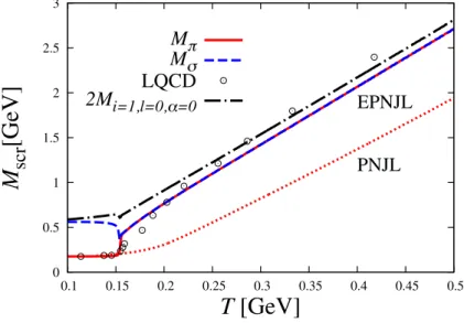
The pion screening mass M

obtained by state-of-the-art 2+1 flavor- LQCD simulations [30] is well analyzed by the present 2-flavor EPNJL model simply, since the meson is composed of u and d quarks only and has no s-quark component. In the LQCD simulations [30], the chiral transition temperature is T

= 196 MeV, although it is T

= 154 ± 9 MeV in finer 2+1-flavor LQCD simulations [40,41] close to the continuum limit. Therefore, we rescale the LQCD results of Ref. [30] with a factor 154/196 in order to reproduce T

= 154 ± 9 MeV. The model parameters, m

and T

, are refitted so as to reproduce the rescaled 2+1-flavor LQCD data, i.e., M

= 175 MeV at vacuum and T

= 154 ± 9 MeV; the resulting values are m

= 10.3 MeV and T

= 156 MeV. The variation of m

from the original value 6.3 MeV to 10.3 MeV little changes the values of σ and Φ.

As shown in Fig. 2.3, the M

calculated with the EPNJL model (solid line) well reproduces the LQCD results (open circles), when α

= α

= 0.31.

In the PNJL model with α

= α

= 0, the model result (dotted line) largely

2.5. NUMERICAL RESULTS 19

0 0.2 0.4 0.6 0.8 1

0.6 0.8 1 1.2 1.4 1.6 1.8 2

σ / σ 0 , Φ

T / T _c

σ/σ

(EPNJL) Φ(EPNJL) σ/σ

(LQCD) Φ(LQCD)

Fig. 2.2: T dependence of chiral condensate and Polyakov loop in the 2-flavor system. In model calculations, we use T

= 200 MeV and α

= α

= 0.2.

LQCD data are taken from Ref. [38] for the chiral condensate and Ref. [39]

for the Polyakov loop. The chiral condensates are normalized by the zero temperature value σ

.

underestimates the LQCD results, indicating that the entangle coupling is

important. The dashed line denotes the sigma-meson screening mass M

obtained by the EPNJL model with α

= α

= 0.31. The solid and dashed

lines are lower than the threshold mass M

(dot-dashed line). This ensures

that the M

and M

determined from the location of the single pole in

the complex-˜ q plane agree with those from the exponential decay of ζ

(0, x)

at large r. The chiral restoration takes place at T ≈ T

= 154 MeV,

since M

= M

there. After the restoration, the screening masses rapidly

approach the threshold mass and finally 2πT . The threshold mass is thus an

important concept to understand T dependence of screening masses.

0 0.5 1 1.5 2 2.5 3

0.1 0.15 0.2 0.25 0.3 0.35 0.4 0.45 0.5

M scr [GeV]

T [GeV]

PNJL EPNJL M

M

LQCD 2M

Fig. 2.3: T dependence of pion and sigma-meson screening masses. In model calculations, we use T

= 156 MeV for the PNJL and EPNJL models. The parameters α

and α

in the EPNJL model are set to α

= α

= 0.31.

LQCD data are taken from Ref. [30] for pion screening mass. M

and M

calculated by the EPNJL model are denoted by the solid and dashed lines, respectively, whereas M

calculated with the PNJL model is shown by the dotted line. The M

obtained by 2+1-flavor LQCD simulations are denoted by the open circles. The dot-dashed line stands for the threshold mass.

2.6 Short Summary

We have proposed a practical method of calculating meson screening masses M

(T ) in NJL-type effective models. The method is based on the following two procedures:

(1) The PV regularization,

(2) A new prescription of calculating the spatial correlation function for meson screening mass.

In the three-dimensional momentum cutoff regularization commonly used, artificial oscillations appear in the spatial mesonic correlation function, since the regularization breaks Lorentz invariance in momentum space. In the PV regularization taken in this thesis, such artificial oscillations do not appear, because the PV regularization possesses Lorentz invariance.

In the previous formalism [35] for the correlation function ζ

(0, x) in

coordinate x space, it is calculated by Fourier transformation from the cor-

relation function χ

(0, q ˜

) in momentum ˜ q space. However, the Fourier

transformation is quite difficult, because it demands ˜ q integration of highly

oscillating function in the long distance limit ( | x | → ∞ ) where the meson

2.6. SHORT SUMMARY 21 screening mass is evaluated. In principle, we can avoid the difficulty by per- forming the Fourier transformation as a contour integral in the complex-˜ q plane. In the previous formalism [35] where the Matsubara summation is taken before the internal-momentum integration in the Fourier transforma- tion, temperature cuts appear near the real-˜ q axis in the complex-˜ q plane and the evaluation of the cuts still demands heavy numerical calculations. In our formalism, we take the Matsubara summation after the internal-momentum integration in the Fourier transformation, and thereby such temperature cuts do not appear. Cuts and a pole appearing in our formalism are located only on the imaginary-˜ q axis in the complex-˜ q plane. We can then obtain the me- son screening mass as a pole of χ

(0, q ˜

), when the pole is located below the cuts. The lowest branch point can be regarded as the threshold mass M

(T ).

Therefore, we can easily evaluate the meson screening mass M

(T ) when M

(T ) < M

(T ).

First, we have proposed the new version of EPNJL model that is based

on the PV regularization instead of the three-dimensional momentum-cutoff

regularization commonly used. We have then applied the prescription (2) to

the EPNJL model in order to analyze T dependence of pion and sigma-meson

screening masses and shown that the model well explains recent 2+1 flavor

LQCD results on T dependence of pion screening mass and the value of T

,

when α

= α

= 0.31 and T

= 156 MeV.

Chapter 3

U (1) _A symmetry restoration

We consider the effective U(1)

-symmetry restoration with the 2+1-flavor EPNJL model. For this purpose, T dependence is introduced for the coupling strength K of the Kobayashi-Maskawa-’t Hooft (KMT) determinant inter- action: K = K (T ). The K(T ) is determined from state-of-the-art LQCD results on T dependence of screening masses for pion and its U (1)

partner (a

meson). The K(T ) thus obtained is strongly suppressed in the vicinity of the pseudocritical temperature of chiral transition. The EPNJL model with the K(T ) well reproduces meson susceptibilities calculated by LQCD simulations. By using this reliable model, we predict light-quark mass (m

) and strange-quark mass (m

) dependence of chiral transition particularly around the physical point (m

, m

) = (6.2 MeV, 175 MeV). We show that the chiral transition is the second order at the “light-quark chiral-limit” point (m

, m

) = (0 MeV, 175 MeV). We find that a tricritical point appears in the southwest direction from the physical point. The location we find is (m

, m

) = (0 MeV, 127 MeV).

3.1 U (1) _A symmetry and Columbia plot

As already mentioned in Sec. 1.1.3, global U(1)

symmetry is explicitly bro- ken by the quantum anomaly through the topologically nontrivial gauge con- figurations (instantons and antiinstantons). At high T , instanton density (dn

(T )) is suppressed by Debye screening in the medium. Pisarski and Yaffe calculated the suppression S(T ) ≡ dn

(T )/dn

(0) perturbatively in high T [42], say T > ∼ 2T

for the pseudocritical temperature T

of chiral transition, and S(T ) was obtained by

S(T ) = exp 3

− π

ρ

T

- 2

3 N

+ 1 3 N

.4

= exp[ − T

/b

] (3.1)

with the instanton radius ρ. The typical value of ρ is about 1/3 fm, and hence the suppression parameter b is about 0.70T

for N

= N

= 3 of

22