スギ・ヒノキ人工林における林分構造が樹幹流に与える影響

(1)

九州大学学術情報リポジトリ

Kyushu University Institutional Repository

スギ・ヒノキ人工林における林分構造が樹幹流に与える影響

鄭, 聖勳

http://hdl.handle.net/2324/4110553

出版情報：Kyushu University, 2020, 博士（農学）, 課程博士バージョン：

権利関係：

(2)

Influence of forest stand structure on stemflow in Japanese cedar and cypress plantations

Seonghun JEONG

Kyushu University

2020

(3)

(4)

Influence of forest stand structure on stemflow in Japanese cedar and cypress plantations

Abstract

Rainfall partitioning (RP) into throughfall (TF), stemflow (SF), and interception loss (IL) largely influences forest ecosystem services such as (1) water resources, (2) disaster prevention, and (3) nutrient cycling. RP should be significantly affected by forest stand structure, and accordingly, understanding the relationship between RP and forest stand structures is required to enhance forest ecosystem services. Researches on TF and IL of RP have widely been conducted in coniferous plantations, and practical estimation models for TF and IL have been developed using common forest inventory data. Although these models are practical, there are still few studies of RP in dense unmanaged coniferous plantations. Some previous studies proposed that some factors other than forest inventory data such as leaf area and dead branches should be considered for RP. In addition to this, there are few studies on SF, possibly because SF had been generally regarded as a small portion of gross rainfall (GR). However, SF could be different and unignorable depending on forest stand structure. Thus, quantification of RP in dense unmanaged forests and understanding and modeling the relationship between SF and forest stand structure are required for providing better forest ecosystem services. The objectives of this study were (1) to clarify the difference of RP in a dense unmanaged coniferous plantation, (2) to find stand structure factors affecting RP in the dense unmanaged coniferous plantations, and (3) to develop SF estimation models for Japanese cedar and cypress plantations for better forest and water management.

First, the study was conducted in a dense unmanaged 32-year-old Japanese cypress plantation with a stand density (SD) of 2500 stems ha⁻¹ at the Takada experimental site in the Kasuya Research Forest, Kyushu University, Fukuoka, Japan. Intensive RP measurements were made over one year from May, 2016 to May, 2017 in a plot (20 m x 10 m), and the measured data were

(8)

ii

compared with the published 36 data of Japanese cedar and cypress plantations in Japan. The results demonstrated that the present RP was markedly different compared with the previous studies (the highest SF/GR: 18.9%, the lowest TF/GR: 47.5%, and the highest IL/GR: 33.6%). This study highlights that RP can significantly differ and SF accounts for a high proportion of RP in unmanaged coniferous plantations with high SD.

Second, to confirm the above result of the high proportion of SF, one more plot (20 m x 10 m) adjacent to the plot (c.a. 50m apart) was established under the same SD of 2500 stems ha^−1, but different stand characteristics. The stand characteristics, including branch structure (live and dead branches), were investigated in detail to determine new stand structure factors. RP was then intensively monitored in the two study plots from April to October 2017 during the growing season.

The results showed that SF/GR ratios were the highest (23.3% and 21.9%) and exceptionally high compared with previous studies with ≤ 2400 stems ha⁻¹. The results also implied that the exceptionally high SF/GR could be induced by the additional gain of rainwater by the dense dead branches but the dead branches effect on generating SF could be limited to the upper dead branches.

To bridge the gap of an absence of SF estimation models of RP, SF/GR estimation models were examined using common forest inventory data and other factors related to forest stand structures. A set of SF/GR and stand structures given in forest inventory data (SD, total basal area, mean diameter at breast height (^DBH ), mean tree height, canopy cover, and leaf area index) was collected from the 25 previous studies of Japanese cedar and cypress plantations and examined with the measured data of this study. To further investigate the relationship between SF/GR and forest stand structures, additional stand structure variables (mean basal area, mean stem surface area, and total stem surface area) derived from the forest inventory data and the stand-scale funneling ratio (FRstand) assessing the efficiency of funneling rainwater were also examined. The

(9)

iii

results showed that among all the stand structure variables, SD exclusively determined SF/GR, providing the best-fitting positive single linear regression equation as a density-based SF/GR model (RMSE = 2.4%). This model is useful for the purpose of practical forest water management because it requires the most common forest inventory data (SD). However, it has a weak point in sustainable forest management because it does not reflect tree growth. Thus, a size-density based SF/GR model (RMSE = 2.0%) was developed on the basis of a strong relationship between FRstand

and ^DBH(R² = 0.845). This model reflects the effects of not only SD but also tree growth by DBH on SF/GR. The size-density based SF/GR estimation model using only common forest inventory data will contribute to the evaluation and control of SF in sustainable forest water management.

This study emphasizes that SF is significantly altered depending on forest stand structure, and thus cannot be always a small portion of GR. The SF estimation models developed in this study could provide better forest ecosystem services together with the existing TF and IL models.

Keywords:

Coniferous plantation; diameter at breast height; forest stand structure; rainfall partitioning; stand density; stemflow

(10)

iv

List of Tables

Chapter 2

Table 2.1 Stand structures of plot 1 (P1) and plot 2 (P2)··· 19 Table 4.1 The differences of TF/GR, SF/GR and IL/GR (ΔTF/GR, ΔSF/GR, and

ΔIL/GR) between plot 1 (P1) and plot 2 (P2) for four GR classes and total GR. Positive values indicate that the ratio in P1 was larger than that in P2 and vice versa. ··· 45 Appendix

Appendix T1 Data for rainfall partitioning (RP) and canopy storage capacity (S) in Japanese coniferous plantations. SD, GR, TF, SF, and IL denote stand density, gross rainfall, throughfall, stemflow, and interception loss, respectively. ··· 86 Appendix T2 Summary of forest stand structure variables (SD: stand density, BA: total

basal area, SA: total stem surface area, 𝐻̅: mean tree height, 𝐷𝐵𝐻̅̅̅̅̅̅: mean diameter at breast height, 𝐵𝐴̅̅̅̅: mean basal area, 𝑆𝐴̅̅̅̅: mean stem surface area) and gross rainfall (GR), throughfall (TF), TF ratio (of GR), stemflow (SF), SF ratio (% of GR), and the stand-scale funneling ratio (FRstand) in the coniferous plantations of Japanese cedar and Japanese cypress in Japan. ··· 88 Appendix T3 Pearson correlation coefficients (r) of (1) stand density (SD), (2) stemflow

ratio (% of gross rainfall (GR), SF/GR) and (3) stand-scale funneling ratio (FRstand) with stand-structure variables (mean tree height (𝐻̅), mean diameter at breast height (𝐷𝐵𝐻̅̅̅̅̅̅), mean basal area (𝐵𝐴̅̅̅̅), mean stem surface area (𝑆𝐴̅̅̅̅), total basal area (BA), total stem surface area (SA), stand density (SD), canopy cover (CC), and leaf area index (LAI)). ··· 90

(11)

v

List of Figures

Chapter 1

Fig. 1.1 The interaction between rainfall partitioning into throughfall (TF), stemflow (SF), and interception loss (IL) and forest canopy in forest ecosystems ··· 2 Fig. 1.2 A comparison between (a) a managed coniferous plantation and (b) an

unmanaged coniferous plantation ··· 4 Fig. 1.3 Relationship between stand density (SD) and interception loss (IL) ratio to

gross rainfall (GR) (IL/GR) for coniferous forests. This figure is drawn based on the data set in Komatsu et al. 2007. ··· 5 Fig. 1.4 Relationship between stand density (SD) and interception loss (IL) ratio to

gross rainfall (GR) (IL/GR) for coniferous forests. This figure is drawn based on the data set in Komatsu et al. 2015. ··· 6 Fig. 1.5 Relationships (a) between stand density (SD) and throughfall (TF) ratio to

gross rainfall (GR) (TF/GR, %), (b) between canopy cover (CC) and TF/GR, and (c) between basal area (BA) and TF/GR for Japanese cedar and cypress plantations. These stand-structure variables were used in Sun et al.

(2017) to develop TF estimation model using multiple-regression analysis (see the TF model equation in Eq. 1.3). This figure is drawn based on the data set in Sun et al. 2017. ··· 7 Fig. 1.6 The roles of stemflow in forest ecosystems ··· 8 Fig. 1.7 Schematic of the role of concentrated stemflow as a source of groundwater

recharge around a tree. Adapted from Tanaka et al. (1996). Hydrological Processes 10, 81−88. ··· 11 Fig. 1.8 36 data of previous studies of Japanese coniferous plantations with

“interception loss (IL)”, “RP” (rainfall partitioning), “throughfall” (TF), and “stemflow (SF)” as a topic. ··· 13 Fig. 1.9 Structure of this study ··· 15

(12)

vi Chapter 2

Fig. 2.1 Location of the Takada experimental site, Kasuya Research Forest, Kyushu University, Japan and photos and measurement designs of the study plot 1, and study plot 2. The black circles indicate trees, the diamonds shapes indicate stemflow measurement, and the white circles indicate funnel-type throughfall collectors.··· 18 Fig. 2.2 Schematic diagrams of branch distribution in the study plot 1 (P1) and

study plot 2 (P2). Nlb and Ndb denote the number of live branches and dead branches, respectively. Each number indicates the average ± standard deviation of the number of branches and thickness of layers with their percentage of the total number of branches or tree height. ··· 21 Fig. 2.3 Gross rainfall measurement using (a) a funnel-type rain collector and (b) a

0.2 mm tipping bucket rain gauge with a data logger (the left rain gauge) in the open space ··· 22 Fig. 2.4 Throughfall measurement using a funnel-type rain collector··· 23 Fig. 2.5 Stemflow measurement with two 90L tanks··· 24 Fig. 2.6 Location of the experimental plots. A numerical with tree species names

(Cedar: Japanese cedar; Cypress: Japanese cypress) denotes the data codes, which are described in Appendix T2. ··· 27 Fig. 2.7 Individual-scale stemflow funneling ratio··· 29 Fig. 2.8 Stand-scale stemflow funneling ratio··· 30 Chapter 3

Fig. 3.1 Relationships between gross rainfall (GR) and throughfall (TF) (a), stemflow (SF) (b), and interception loss (IL) (c), and between GR and TF/GR (d), SF/GR (e), and IL/GR (f), respectively. ···

37 Fig. 3.2 The relationship between throughfall (TF) and gross rainfall (GR).

Canopy storage capacity (S) was obtained using the minimum method.

The dashed line and the solid line denote 1:1 line and the upper envelope line, respectively. ···

37

(13)

vii

Fig. 3.3 Comparison of each of throughfall (TF), stemflow (SF), and interception loss (IL) to gross rainfall (GR) with previous studies of coniferous plantations in Japan. Boxplots indicate the previous studies and black circles indicate the present study. ··· 38 Fig. 3.4 Relationships (a) between the stand density (SD) and stemflow (SF) ratio

of gross rainfall (GR) (SF/GR) and (b) between SD and the mean SF volume of the individual tree per unit gross rainfall (SFind). The triangles and blue circles denote the previous studies in Japanese coniferous plantations and the present values in this study, respectively. ···

40 Chapter 4

Fig. 4.1 Relationships between gross rainfall (GR) and each component of RP on a weekly basis: (a) TF, (b) SF, and (c) IL. Open and solid circles indicate data from the study plot 1 (P1) and study plot 2 (P2), respectively. The solid and dashed lines indicate the linear regression lines of P1 and P2 determined by the least-squares method, respectively. ···

44 Fig. 4.2 Relationships between the stand density (SD) and the ratios of each

component of rainfall partitioning (RP) to gross rainfall (GR) in this study with previous studies of Japanese coniferous plantations (n = 36): (a) TF/GR, (b) SF/GR, and (c) IL/GR. The triangles denote the ratios in previous studies. The blue and red circles denote the ratio in study plot 1 and the ratio in study plot 2, respectively. The solid lines are the regression lines determined by the least-squares method. ···

46 Fig. 4.3 Relationships between gross rainfall (GR) and throughfall (TF) on a

weekly basis in the (a) study plot 1 and (b) study plot 2, respectively. The solid lines are the upper envelope lines for estimating canopy storage capacity (S). ···

47 Fig. 4.4 Relationships (a) between the average number of dead branches (Ndb) and

the ratio of throughfall to gross rainfall (TF/GR) and (b) between the average dead branch space (sdb) and TF/GR for the 16 subplots, respectively. The white and black circles indicate the data in the study plot 1 and study plot 2, respectively. The solid line indicates the regression line determined by the least-squares method.

48 Fig. 4.5 Relationships (a) between the number of dead branches (Ndb) and the

individual funneling ratio (FRi) and (b) between the dead branch space (sdb) and FRi. The open and solid circles indicate the study plot 1 and study plot 2, respectively. ··· 49

(14)

viii Chapter 5

Fig. 5.1 Relationships between stand density (SD) and (a) mean tree height (𝐻̅), (b) mean diameter at breast height (𝐷𝐵𝐻̅̅̅̅̅̅), (c) mean basal area (𝐵𝐴̅̅̅̅), (d) mean stem surface area (𝑆𝐴̅̅̅̅), (e) total basal area (BA), (f) total stem surface area (SA), (g) canopy cover (CC), and (h) leaf area index (LAI). Squares denote the data of no management since planting, and circles denote the data of several years after thinning. Triangles denote the data of right after thinning. The red arrows show the change from right before thinning to right after thinning. The solid line and dotted lines show the regression lines that were fitted to all data and the data without the right-after-thinning data, respectively. The Pearson correlation coefficient and its p-value are provided in Appendix T3. ···

63 Fig. 5.2 Relationships between the ratio of stemflow (SF) to gross rainfall (GR)

(SF/GR) and (a)mean tree height (𝐻̅), (b) mean diameter at breast height (𝐷𝐵𝐻̅̅̅̅̅̅), (c) mean basal area (𝐵𝐴̅̅̅̅), (d) mean stem surface area (𝑆𝐴̅̅̅̅), (e) total basal area (BA), (f) total stem surface area (SA), (g) stand density (SD), (h) canopy cover (CC), and (i) leaf area index (LAI). Squares denote the data of no management since planting, and circles denote the data of several years after thinning. Triangles denote the data of right after thinning. The red arrows show the change from right before thinning to right after thinning. The solid line and dotted lines show the regression lines that were fitted to all data and the data without the right-after-thinning data, respectively. The Pearson correlation coefficient and p-value are provided in Appendix T3. ···

66 Fig. 5.3 Comparison between the estimated and observed ratio of stemflow (SF) to

gross rainfall (GR) (SF/GR) derived from the data set of this study. The SF/GR ratio was estimated by the Eq. (5.7). Squares denote the data of no management since planting and circles denote the data of several years after thinning. Triangles denote the data of right after thinning. The broken line is the 1:1 line. ···

67

(15)

ix

Fig. 5.4 Simulation results for the two stemflow estimation models over the possible ranges of tree growth in Japanese cedar and cypress plantations with different stand densities (SDs). The panels (a) and (b) are the results of the single regression model of the ratio of stemflow (SF) to gross rainfall (GR) (SF/GR) with SD and the multiple regression model of SF/GR ratio with SD and total basal area (BA), respectively. The solid lines plot the possible changes in SF/GR ratio against mean diameter at breast height (𝐷𝐵𝐻̅̅̅̅̅̅) in virtual Japanese cedar and cypress plantations with different SDs (500, 1500, and 2500 stems ha⁻¹). ···

69 Fig. 5.5 Relationships between the stand-scale funneling ratio (FRstand) and (a)

mean tree height (H̅), (b) mean diameter at breast height (𝐷𝐵𝐻̅̅̅̅̅̅), (c) mean basal area (𝐵𝐴̅̅̅̅), (d) mean stem surface area (𝑆𝐴̅̅̅̅), (e) total basal area (BA), (f) total stem surface area (SA), (g) stand density (SD), (h) canopy cover (CC), and (i) leaf area index (LAI). Squares denote the data of no management since planting, and circles denote the data of several years after thinning. Triangles denote the data of right after thinning. The red arrows show the change from right before thinning to right after thinning.

The solid line and dotted lines show the regression lines that were fitted to all data and the data without the right-after-thinning data. The Pearson correlation coefficient and p-value are provided in Appendix T3. ···

71 Fig. 5.6 Relationship between the stand-scale funneling ratio (FRstand) and mean

diameter at breast height ( 𝐷𝐵𝐻̅̅̅̅̅̅ ). Squares denote the data of no management since planting, and circles denote the data of several years after thinning. Triangles denote the data of right after thinning. The red arrows show the change from right before thinning to right after thinning.

73 Fig. 5.7 Comparison between the estimated and observed ratio of stemflow (SF) to

gross rainfall (GR) (SF/GR) derived from the data set of this study. The SF/GR ratio was estimated by Eq. (5.12). Squares denote the data of no management since planting, and circles denote the data of several years after thinning. Triangles denote the data of right after thinning. The broken line is the 1:1 line. ···

74

(16)

x

Fig. 5.8 Simulated relationships of total basal area (BA) and stand-scale funneling ratio (FRstand) with the mean diameter at breast height (𝐷𝐵𝐻̅̅̅̅̅̅) and between the ratio of stemflow (SF) to gross rainfall (GR) (SF/GR) and 𝐷𝐵𝐻̅̅̅̅̅̅ of virtual Japanese cedar and cypress plantations with different stand densities (SDs) by the size-density based SF/GR model. The solid and dashed lines in the panel (a) show the possible changes in BA and FRstand versus 𝐷𝐵𝐻̅̅̅̅̅̅, respectively. The solid lines in the panel (b) show the possible changes in SF/GR versus 𝐷𝐵𝐻̅̅̅̅̅̅ with different SDs (500, 1500, and 2500 stems ha⁻¹). · 75 Chapter 6

Fig. 6.1 Comparison between annual average SF/GR (%) and the SF/GR (%) of heavy rainfall. This figure is drawn using the rainfall partitioning data obtained from the study plot 1. ··· 80

(17)

xi

List of Abbreviations and Acronyms

Abbreviation Descriptor Unit

Astand The stand area m²

Aha The unit area 10000 m² ha⁻¹

BA Basal area m² ha⁻¹

BAi Basal area of the observed trees m²

BAstand The total basal area of the stand m²

𝐵𝐴̅̅̅̅ Mean basal area m²

CC Canopy cover ratio %

CFTF Free throughfall coefficient −

CPA Crown projection areas m²

CV Coefficient of variation −

DBH Diameter at breast height cm

FRind The ratio of the stemflow volume to the hypothetical

rainwater on basal area at the individual-scale − FRstand The ratio of the stemflow volume to the hypothetical

rainwater on basal area at the stand-scale −

GR Gross rainfall mm

H Tree height m

IL Interception loss mm

IL/GR Ratio of interception loss to gross rainfall %

LAI Leaf area index m² m⁻²

nc The number of throughfall collectors −

ntree The number of stemflow observed trees −

Ntree The total number of trees in the plot −

Ndb The number of dead branches −

Nlb The number of live branches −

p Significant level %

(18)

xii

Abbreviation Descriptor Unit

P1 Plot 1 m²

P2 Plot 2 m²

PA Plot area m²

PAI Plant area index m² m⁻²

RP Rainfall partitioning −

Rs Relative spacing index %

Ry Relative yield index −

S Canopy storage capacity mm

SA Total stem surface area m² ha⁻¹

𝑆𝐴̅̅̅̅ Mean stem surface area m²

S.D. Standard deviation −

SD Stand density stems ha⁻¹

SF Stemflow mm

SF/GR Ratio of stemflow to gross rainfall % SFVi The stemflow volume of the stemflow observed trees L

SFVstand The stemflow volume of the stand L

SV Stand volume m³ ha⁻¹

t Student`s t-value −

TF Throughfall mm

TF/GR Ratio of throughfall to gross rainfall % 𝑁_𝑙𝑏

̅̅̅̅ The average length of live branches −

𝑁_𝑑𝑏

̅̅̅̅̅ The average number of dead branches −

𝑛_𝑑𝑏

̅̅̅̅̅ The average number of dead branch per unit length − 𝑠_𝑑𝑏

̅̅̅̅ Vertical dead branch space cm

ε The error of mean throughfall %

(19)

1

Chapter 1 Introduction

(20)

2

1.1 What is rainfall partitioning in forest ecosystems?

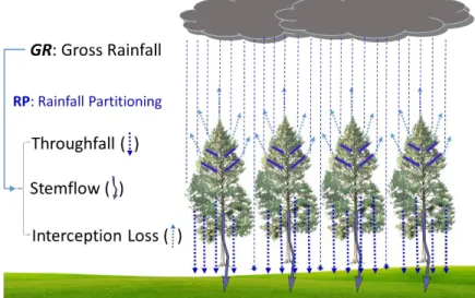
In forest ecosystems, a forest canopy interacts with rainfall and the interactions during storms result in three general hydrologic processes: a water output which goes back to the atmosphere (canopy interception loss, IL) and two water inputs that route rainwater to the forest floor: (1) throughfall (TF) which passes through the canopy or directly falls down to the forest floor and (2) stemflow (SF) which is entrained by the canopy and flows down branches and a stem, known as spatially-localized input around a tree (Fig. 1.1). These processes partitioned by the canopy are termed “rainfall partitioning (RP)”.

RP largely influences forest ecosystems: (1) water resources, e.g., rainfall-to-discharge flow path (Sadeghi et al., 2018) and groundwater recharge, e.g., (Taniguchi et al., 1996; Tanaka, 2011); (2) disaster prevention, e.g., overland flow and soil erosion (Hertwitz, 1986; Liang et al., 2009); and (3) nutrient cycling, e.g., vegetation-solute-soil-root (Zhang et al., 2013 and Levia and Germer, 2015b).

Fig. 1.1. The interaction between rainfall partitioning into throughfall (TF), stemflow (SF), and interception loss (IL) and forest canopy in forest ecosystems.

(21)

3

1.2 Rainfall partitioning in Japanese coniferous plantations

(1) Chronological rainfall partitioning studies: A brief review

The first study on RP was conducted by Robert Horton and achieved a global attention in pre-20^th century (Horton 1919). Since then, many RP studies were conducted across the world. There are several review paper of RP, including all of IL, TF, and SF (Domingo and Llorens, 2007; Barbier et al., 2009; Magliano et al., 2019; Freisen and Van Stan, 2019). Also, there are several review papers which focused on a single component of RP: (1) IL review paper (Muzylo et al., 2009), TF review papers (Levia and Frost, 2006; Levia et al., 2017), and SF review papers (Levia and Frost, 2003; Levia and Germer, 2015; Van Stan 2018).

In Japan, Iwatubo and Tsutsumi (1967) first reported a RP study in an old-aged Japanese cypress plantation, mainly focusing on hydro-chemical fluxes. Since then, many RP studies were actively conducted across Japan, mainly Japanese coniferous plantations (see the data sets from recent studies, IL: Komatsu et al., 2015; TF: Sun et al., 2017; SF: Jeong et al., 2020). There is no review paper of RP, including all of IL, TF, and SF. There is only one review paper focusing on a single component of SF for Japanese forests, including 10 data of Japanese coniferous plantations (Ikawa 2007).

(2) Relationship between rainfall partitioning and forest stand structure

Previous studies addressed that RP is a complex process controlled by a variety of factors such as meteorological conditions, e.g., evaporation rate, rainfall intensity, and rainfall amount (Gash, 1979; Llorens et al., 1997; Komatsu et al., 2008) and forest stand structures, e.g., stand density (SD), basal area (BA), and canopy cover (CC) (Teklehaimanot et al., 1991; Komatsu et al., 2007,

(22)

4

2015; Molina and del Campo, 2012; Sun et al., 2015; Sun et al., 2017). The examination of RP in the regions where climate conditions (e.g., annual precipitation, seasonality of precipitation) are comparable, however, could reduce the effects of the climate conditions and enable us to investigate the effects of forest stand structures with similar phenology on RP (Komatsu et al., 2007, 2015; Sun et al., 2017).

In Japan, forests cover approximately 67% of the total land, of which 41% is occupied by plantations (Japan Forestry Agency, 2017). Japanese cedar (Cryptomeria japonica D. Don) and Japanese cypress (Chamaecyparis obtusa Endl.) were the two dominant tree species occupying 44% and 25% of the plantations, respectively. A substantial number of these coniferous plantations have not been managed on account of the economic recession on forestry since the 1980s (Onda et al., 2010; Fig. 1.2). Accordingly, these coniferous plantations have been kept under high stand density (SD) and densely covered by canopies. These unmanaged plantations tend to (1) intercept more

rainwater at the canopies and thus reduce water supply to the forest floor (Kuraji, 2003; Sun et al., 2015; Shinohara et al., 2015) and (2) have little or no understory due to little sunlight passing through the canopies, which could result in increased loss of surface soil and nutrients (Nanko et al., 2016) and increasing flooding and soil erosion (Shinohara et a., 2015).

Fig. 1.2. A comparison between (a) a managed coniferous plantation and (b) an unmanaged coniferous plantation.

(23)

5

Komatsu et al. (2015) highlighted the usefulness of SD as a key forest stand structure for Japanese coniferous plantations. Sun et al. (2017) evaluated SD, canopy cover (CC), and basal area (BA) as the useful forest stand structure factors for TF in Japanese coniferous plantations in Japan, among which SD was most highly related to TF.

(3) Modelling rainfall partitioning

For forest ecosystem services in Japanese coniferous plantations with the two dominant plantation species, Komatsu et al. (2007, 2015) and Sun et al. (2017) developed IL and TF estimation models using common forest inventory data as follows.

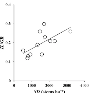
For the IL estimation model, Komatsu et al. (2007) found a tight correlation between SD and IL/GR with 12 data set of coniferous plantations, among which the 12 data set includes three Pinus densiflora plantations (Fig. 1.3). The model equation was obtained as follows:

IL/GR = 0.00498 SD + 12.0 (1.1)

Fig. 1.3. Relationship between stand density (SD) and interception loss (IL) ratio to gross rainfall (GR) (IL/GR) for coniferous forests. This figure is drawn based on the data set in Komatsu et al.

2007.

(24)

6

Komatsu et al. (2015) further developed the IL/GR model by amplifying the data set (n = 46) (Fig. 1.4). In this model, the authors excluded the three data of the Pinus densiflora plantations and used the two dominant plantation species (Japanese cedar and cypress) solely. The model equation was obtained as follows:

IL/GR = 0.308 {1 – exp (−0.000880 * SD)} (1.2)

This model has a typical error of 4%.

For the TF estimation model, Sun et al. (2017) found key stand-structure variables (SD, CC, and BA) (Fig. 1.5), which had an impact on TF and developed TF estimation models for Japanese cedar and cypress plantations as follows:

TF/GR (%) = −0.0219×SD – 0.2818×SD + 0.1388×BA + 103.0985 (1.3) This model has a relative error of 3.2 ± 2.4%.

Fig. 1.4. Relationship between stand density (SD) and interception loss (IL) ratio to gross rainfall (GR) (IL/GR) for coniferous forests. This figure is drawn based on the data set in Komatsu et al.

2015.

(25)

7

These two models for estimating IL and TF have been used to evaluate the effects of forest stand structure on the forest water cycle (Dung et al., 2011, 2012a, b; Shinohara et al., 2015; Jeong et al., 2019b).

(4) Research gaps of rainfall partitioning

Although these two models are practical, there still remains gaps in RP studies for Japanese coniferous plantations. First, the dataset in the above-mentioned Japanese coniferous plantations includes the data with various SD; however, there are few data with a SD at ≥ 2500 stems ha⁻¹ which is a typical planting density for the Japanese coniferous species (Japan Forestry Agency, 2017). Second, Shinohara et al. (2010) addressed that there was a possibility of appearing new stand structure factors affecting RP such as leaf area and dead branches in dense unmanaged coniferous plantations other than SD. Third, less attention to SF has been paid, possibly due to the small proportion of GR; however, SF could greatly depend on forest stand structure (Levia and Frost, 2003; Levia and Germer, 2015b; Carlyle-Moses et al., 2018; Van Stan and Gordon, 2018).

Fig. 1.5. Relationships (a) between stand density (SD) and throughfall (TF) ratio to gross rainfall (GR) (TF/GR, %), (b) between canopy cover (CC) and TF/GR, and (c) between basal area (BA) and TF/GR for Japanese cedar and cypress plantations. These stand-structure variables were used in Sun et al. (2017) to develop TF estimation model using multiple-regression analysis (see the TF model equation in Eq.

1.3). This figure is drawn based on the data set in Sun et al. 2017.

(26)

8

Therefore, finding the relationships between all the components of RP and key stand structure factors in addition to SD, CC and BA including the data with a SD at 2500 stems ha⁻¹ or more and developing SF estimation models for Japanese coniferous plantations as well as IL and TF is required for better understanding of RP and better effective forest ecosystem services.

1.3 Important role of stemflow in forest ecosystems

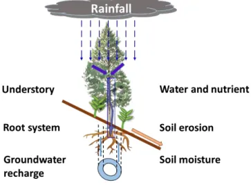
Although the quantitative SF/GR has reportedly been ignorable (Van Stan and Gordon, 2018), many previous studies on SF found that SF exerts an important role in forest ecosystems. This sub- section explains the important role of SF in a viewpoint of forest ecosystem services (Fig. 6).

Water and hydro-chemical fluxes

SF is generally evaluated as a portion of GR (SF/GR) and regarded as a minor portion of GR;

however, SF hydro-chemical fluxes could be much higher (Levia and Frost, 2003; Levia and Germer, 2015). For example, Liu et al. (2003) reported that SF/GR was only 2%, whereas SF

Fig. 1.6. The roles of stemflow in forest ecosystems.

(27)

9

contributed approximately 10% of mineral nitrogen. Also, Levia and Germer (2015) reported that for forests with SF accounting for around 5% of GR, 10~20% of total fluxes is commonly contributed by SF. Thus, the small portion of GR cannot imply that SF hydro-chemical fluxes are also low.

There is an only one SF review paper which collected previous studies of Japanese forests (Ikawa 2007). The author emphasized the importance of SF chemistry associated with acid rain, mostly resulted from atmospheric deposition by anthropogenic activities. The high SF acidity in coniferous plantations was confirmed to acidify the soil around a stem as a spatially-localized input of SF rainwater, which could seriously threaten the coniferous plantations. Since Japanese coniferous plantations have been poorly managed as aforementioned, the problem might be more seriously increased.

Understory vegetation

The SF of understory vegetation has been emphasized since it funnels considerable amount of rainwater down to the forest floor (e.g., Manfroi et al., 2004; Germer et al. 2010; González- Martínez et al., 2016; Gordon et al., 2019). SF is enriched in a number of elements including N (Langkamp et al. 1982). Thus, it is generally believed that SF hydro-chemical fluxes could stimulate tree growth, while the delivery of allelopathic chemicals in SF may hamper the growth of understory vegetation and nearby woody trees (May and Ash, 1990).

Root and microbial community

Stemflow-induced preferential flow along roots, termed “double-funneling of stemflow” has been reviewed by Johnson and Lehman (2006). Some previous studies in the review paper showed that

(28)

10

preferential SF occurred next to roots (Martinez-Meza and Whitford, 1996; Li et al., 2009). Since the review paper, Rosier et al. (2015) delved into potential impacts of SF, including TF, on root and microbial community. The authors hypothesized that SF may affect root symbiotic bacteria (root nodule N-fixing bacteria) and mycorrhizal fungi (eco- and endomycorrhiza) since SF could supply roots with water and nutrients.

Soil moisture

SF rainwater infiltrates and contribute great water input into the soil (Liang et al., 2007; Liang et al., 2011; Návar, 2011), which may partly be available for tree growth. Soil moisture by SF is heterogeneous and the patterns of soil moisture can be influenced by topography, resulting in a greater soil moisture increase downslope of stems compared with upslope of stems (Liang et al., 2007). Liang et al. (2011) found that soil water depletion for tall stewartia (Stewartia monadelpha) on a hillslope was higher for a period with SF compared to one without SF, probably because of drainage. The heterogeneity could be reduced by forest operations (e.g., thinning or clearing) because of the decreased localized input of SF rainwater (Levia and Germer, 2015).

Groundwater recharge

Hitherto, to my knowledge, there have been very few previous studies that address ground water recharge induced by SF (Taniguchi et al., 1996; Tanaka, 2011). Taniguchi et al. (1996) reported that SF/GR in two pine forests (Pinus densiflora Sieb. et Zucc) accounted for 0.5% and 1.2%, respectively, whereas the SF contributed 10.9% and 19.1% to the total annual ground recharge.

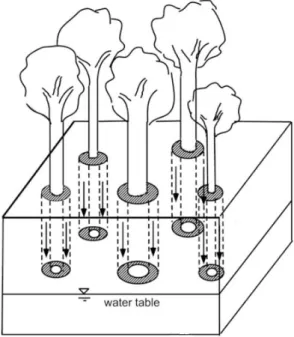
Tanaka et al. (1996) accounted for stemflow-induced groundwater recharge using a cylindrical infiltration model, which is related to the tree diameter (Fig. 1.6).

(29)

11

Therefore, SF could be a driver for localized deep percolation and groundwater recharge and greatly contribute to the annual groundwater recharge in some regions where SF/GR is very high. Further researches should be quantitatively conducted in Japanese coniferous plantations to assess the changes in groundwater recharge by forest stand structure.

Overland flow and Soil erosion

Herwitz (1986) reported infiltration-excess overland flow by SF in the montane tropical rainforest, northeast Queensland, Australia. The author suggested the similar overland flow could occur in extreme rainfall events. Charlier et al. (2009) reported that runoff model was performed better with SF than that without SF. Bui and Box (1992) reported that stemflow-induced soil erosion was negligible, compared to that of TF for corn and sorghum (e.g.,); Keen et al. (2010) reported that soil erosion is a serious problem induced by SF, accounting for 7% of GR and 6.5 mm m⁻² of soil per year, from Macadamia orchards of southeast Australia. This results promoted the government

Fig. 1.7. Schematic of the role of concentrated stemflow as a source of groundwater recharge around a tree. Adapted from Tanaka et al.

(1996). Hydrological Processes 10, 81−88.

(30)

12

for decision-making of silvicultural regimes that SF trees should be substantially less planted to prevent from soil erosion. Zhao et al. (2020) examined the effect of SF on soil erosion under simulated maize-planted and rainfall conditions and found that SF significantly increased the soil erosion when the rainfall intensities increased, compared with a control. Therefore, the impact of SF on overland flow and soil erosion greatly depends on the SF amount in some regions where experience extreme rainfall events and plantation tree species.

1.4 Scant stemflow studies in Japanese coniferous plantations

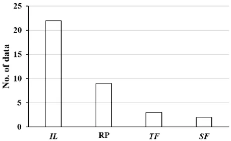
The primary emphasis of this sub-section is to determine what purpose RP studies have been done in Japanese coniferous plantations. For this, the previous studies reporting all of IL, TF, and SF in Japanese coniferous plantations were reviewed and 36 data sets in total were obtained (Fig. 1.8). Most of the studies have been IL with a main purpose of water resources (n = 22), followed by RP (n = 9) for the change in RP by an understory and abandoned plantation, TF (n = 3) for water resources and spatial variability, and SF (n = 2) for chemical-fluxes. Thus, there still have been very few SF studies though SF plays an important role in forest ecosystems as mentioned in section 1.3.

(31)

13 1.5 Objectives of this study

The objectives of this thesis were as follows:

 to clarify the difference of RP in an unmanaged Japanese coniferous plantation (Chapter 3)

 to find stand structure factors affecting RP in dense unmanaged Japanese coniferous plantations (Chapter 4)

 to develop SF estimation models for Japanese coniferous plantations using common forest inventory data (Chapter 5)

In Chapter 2, all materials and methods of this thesis are integrated. First, the characteristics of the study site were described. Second, the measurements of RP and stand structures, including branch structures, were elaborated. Third, data analyses are described. Lastly, SF estimation model developments using the field data of RP obtained from this study and the previous data of previous

Fig. 1.8. 36 data of previous studies of Japanese coniferous plantations with “interception loss (IL)”, “RP” (rainfall partitioning), “throughfall”

(TF), and “stemflow (SF)” as a topic.

(32)

14

studies of Japanese coniferous plantations and model simulation using the data created within a possible range of tree growth in the Japanese coniferous plantations are explained.

In Chapter 3, RP into TF, SF, and IL was monitored in a dense unmanaged Japanese cypress plot with a SD of 2500 stems ha⁻¹ (Plot 1). The present data of each component obtained from the plot were compared with previous studies of Japanese coniferous plantations with a wide range of SD (356−2400 stems ha⁻¹).

In Chapter 4, the intensive monitoring of RP was expanded by establishing one more plot near the plot 1 to confirm the high SF proportion obtained in Chapter 3. Forest stand structures including branch structures (live branches + dead branches) were investigated in detail to address an issue of unmanaged Japanese coniferous plantations and determine a new stand-structure factor influencing SF.

In Chapter 5, based on the results from Chapter 3 and 4, a set of stand-structure variables and SF/GR were collected. The relationships between the stand-structure variables and SF/GR were examined. SF estimation models were developed through single and multiple regression analyses. To confirm the actual changes in SF/GR, the models developed were verified through model simulation.

In Chapter 6, lastly, the synthesized findings from each of the preceding chapters are discussed and the conclusions of this study are provided.

(33)

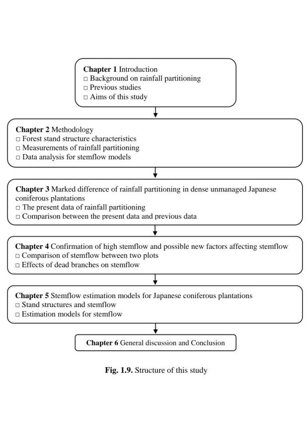
15 Chapter 1 Introduction

□ Background on rainfall partitioning

□ Previous studies

□ Aims of this study

Chapter 3 Marked difference of rainfall partitioning in dense unmanaged Japanese coniferous plantations

□ The present data of rainfall partitioning

□ Comparison between the present data and previous data

Chapter 4 Confirmation of high stemflow and possible new factors affecting stemflow

□ Comparison of stemflow between two plots

□ Effects of dead branches on stemflow

Chapter 5 Stemflow estimation models for Japanese coniferous plantations

□ Stand structures and stemflow

□ Estimation models for stemflow

Chapter 6 General discussion and Conclusion Chapter 2 Methodology

□ Forest stand structure characteristics

□ Measurements of rainfall partitioning

□ Data analysis for stemflow models

Fig. 1.9. Structure of this study

(34)

16

Chapter 2 Methodology

(35)

17 2.1 Study site

This study was conducted in an unmanaged Japanese cypress (Chamaecyparis obtusa Endl.) plantation at the Takada Experimental Site in the Kasuya Research Forest, Kyushu University, Fukuoka, Japan (33°37ʹ58ʹʹ N, 130° 31ʹ 48ʹʹ E, ca 100 m a.s.l.). The plantation has not been managed since planting with a SD of 2500 stems ha⁻¹in 1985. The soil type is brown forest soil originated from serpentine bedrock (Kinoshita et al., 1936). The mean annual temperature and the mean precipitation were 17.1 °C and 1634.3 mm, respectively, recorded from 1986 to 2015 at a meteorological station 9 km southwest of the study site. Rainy season is from June to September, and snowfall rarely occurs.

First, a 20 m × 10 m study plot was established (study plot 1, Fig. 2.1). The understory vegetation was sparse. The slope was relatively steep (26°). SD was equivalent to the initial planting density (2500 trees ha⁻¹), therefore the plot contained 50 trees of Japanese cypress among which five trees had no leaves due to self-thinning.

One more 20 m × 10 m study plots were established (study plot 2, Fig. 2.1). They were approximately 50 m apart (hereafter P1 and P2). SD of this plot was also 2500 stems ha⁻¹ containing 50 trees of Japanese cypress among which five trees had also no leaves due to self- thinning (Fig. 2.1).

(36)

18

Fig. 2.1 Location of the Takada experimental site, Kasuya Research Forest, Kyushu University, Japan and photos and measurement designs of the study plot 1, and study plot 2. The black circles indicate trees, the diamonds shapes indicate stemflow measurement, and the white circles indicate funnel-type throughfall collectors.

(37)

19

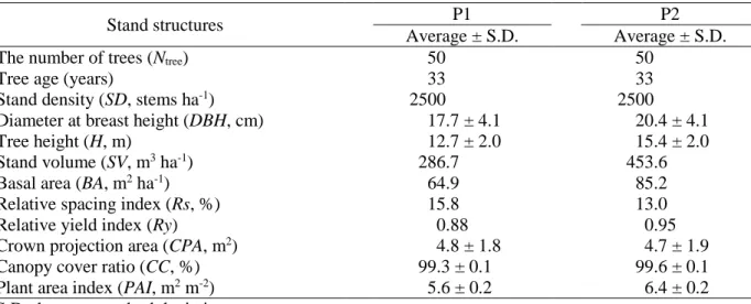
The stand structures of the two plots are summarized in Table 2.1 and the branch structure obtained from all trees of the two plots (n = 50 each) is shown in Fig. 2.2. The recommended BA, relative spacing (Rs), and relative yield index (Ry) indicating status of stocking for silvicultural practice of Japanese cedar and cypress plantations in Japan are 50 m² ha⁻¹, 20%, and 0.7, respectively (Tange and Koike, 2016). Those variables in the plots were 65−85 m² ha⁻¹, 13−16%, 0.88−0.95, respectively, which implies that both plots were overstocked. CC and plant area index (PAI), the variables indicating the status of canopy coverage by leaves, branches, and stems, were 99.3−99.6% and 5.6−6.4 m² m⁻², respectively, which implies that both plots were almost fully covered by the canopies. Considering these variables, P2 was slightly denser than that of P1 (Fig.

2.2, Table 2.1). Tree height and diameter at breast height (DBH), the variables indicating tree size, were 19−20 m and 13−15 cm, respectively, which indicates the tree size in P2 belongs to the highest class and that in P1 belongs to the middle class in the stand of their age in this area (Japan Forestry Agency, 1957).

Table 2.1. Stand structures of plot 1 (P1) and plot 2 (P2)

Stand structures P1 P2

Average ± S.D. Average ± S.D.

The number of trees (Ntree) 50 50

Tree age (years) 33 33

Stand density (SD, stems ha^-1) 2500 2500

Diameter at breast height (DBH, cm) 17.7 ± 4.1 20.4 ± 4.1

Tree height (H, m) 12.7 ± 2.0 15.4 ± 2.0

Stand volume (SV, m³ ha^-1) 286.7 453.6

Basal area (BA, m² ha^-1) 64.9 85.2

Relative spacing index (Rs, %) 15.8 13.0

Relative yield index (Ry) 0.88 0.95

Crown projection area (CPA, m²) 4.8 ± 1.8 4.7 ± 1.9

Canopy cover ratio (CC, %) 99.3 ± 0.1 99.6 ± 0.1

Plant area index (PAI, m² m^-2) 5.6 ± 0.2 6.4 ± 0.2

S.D. denotes standard deviation.

Rs indicates that the ratio of the mean distance between trees to the mean dominant tree height of the stand.

(38)

20

The crown and live branch structures are given in Table 2.1 and Fig. 2.2. The average crown projection area (CPA) was 4.8 m² in P1 and 4.7 m²in P2 and the average crown length was 2.8 in P1 and 3.0 m in P2. The average number of live branches (𝑁̅̅̅̅_𝑙𝑏) and thickness of live branch layer were 15.7 branches (21.8% of the total number of branch) and 2.8 m (22.3% of the tree height) in P1 and 14.7 branches (23.6% of the total number of branch) and 3.0 m (19.5% of the tree height) in P2, respectively. The average number of live branches per unit length (𝑛̅̅̅̅) and _𝑙𝑏 vertical live branch space (𝑠̅̅̅̅) were 5.6 branches m_𝑙𝑏 ⁻¹ and 0.18 m in P1 and 4.9 branches m⁻¹ and 0.20 m in P2, respectively. The results show that the crown and live branch structures were almost identical.

The dead branch structure is shown in Fig. 2.2. Since the trees in the plantation have not been pruned and dead branches of Japanese cypress tend not to fall naturally (Otake et al., 2007), the dead branches were densely distributed from the base of the crown to the nearby forest floor in each plot. The average number of dead branches (𝑁̅̅̅̅̅_𝑑𝑏) and length of dead branch layer were 56.3 branches (78.2% of the total number of branch) and 7.9 m (62.1% of the tree height) in P1 and 47.4 branches (76.4% of the total number of branch) and 10.6 m (68.8% of the tree height) in P2, respectively. The average number of dead branches per unit length (𝑛̅̅̅̅̅) and vertical dead _𝑑𝑏 branch space (𝑠̅̅̅̅) were 7.1 branches m_𝑑𝑏 ⁻¹ and 0.14 m in P1 and 4.5 branches m⁻¹ and 0.22 m in P2, respectively. The results show that the dead branches in P1 were more densely and closely distributed than those in P2, despite the fact that the canopy in P1 was slightly sparser than that in P2 (Table 2.1).

(39)

21 2.2 Forest stand structure measurements

CC and PAI were measured using a pair of LAI-2000 plant canopy analyzers (Li-COR Inc., Lincoln, NE, USA) and FV-200 (LI-COR). The measurements were conducted on an overcast day to avoid the disturbance from direct sunlight. The free TF coefficient (CFTF) was calculated using the following equation (Carlyle-Moses and Price, 1999; Shinohara et al., 2015):

CFTF = 1 – CC (2.1)

In this study, we regarded the visually detectable branches longer than about 50 cm with leaves as live branches and those without leaves as dead branches. Branch distribution was

Fig. 2.2. Schematic diagrams of branch distribution in the study plot 1 (P1) and study plot 2 (P2). Nlb and Ndb denote the number of live branches and dead branches, respectively. Each number indicates the average ± standard deviation of the number of branches and thickness of layers with their percentage of the total number of branches or tree height.

(40)

22

observed by counting the number of live and dead branches using a telescope and measuring the heights of tree top, lowest live branch, and lowest dead branch using a hypsometer (Haglőf Vertex IV-360, Haglőf Inc., Madison, MS, USA).

2.3 Measurements

2.3.1 Gross rainfall measurement

GR was measured using a funnel-type rain collector (funnel diameter = 210 mm) and a HOBO RG3-M tipping bucket rain gauge with a resolution of 0.2 mm (diameter = 154 mm, Onset Computer, Bourne, MA, USA) connected to an Onset HOBO Event data logger installed at a 2 m tower in an open space approximately 50 m apart from each plot (Fig. 2.1; Fig. 2.3). The funnel- type GR was measured on a weekly basis and was strongly correlated to that of the tipping bucket rain gauge (R² = 0.999, p = 0.000); thus, data from the funnel-type rain collector were used in this study.

Fig. 2.3. Gross rainfall measurement using (a) a funnel-type rain collector and (b) a 0.2 mm tipping bucket rain gauge with a data logger (the left rain gauge) in the open space.

(41)

23 2.3.2 Throughfall measurement

TF was measured using 30 funnel-type rain collector which is the same for GR in each plot (Fig. 2.1; Fig. 2.4). They were randomly allocated on the forest floor and maintained throughout the study period. TF (mm) was calculated as follows:

𝑇𝐹 =^{∑ 𝑇𝐹}^𝑖

𝑛𝑐 (2.2) where TFi is the throughfall (mm) of TF collector i and nc is the number of TF collectors.

The data from two TF rain collectors in P1 that normally exceeded GR were excluded for analysis because these TF collectors were placed ≤10 cm from the inclined stems with rough bark and collected not only TF but also separating SF (Levia et al., 2010; Saito et al., 2013). Thus, nc

for P1 and P2 were 28 and 30, respectively. The standard relative errors of mean TF estimated using the following equation (Kimmins, 1973; Saito et al., 2013; Shinohara et al., 2013; Sun et al., 2014) for P1 and P2 were 5.0% and 5.4%, respectively:

𝜀 = (𝑡 × 𝐶𝑉)/√𝑛𝑐 (2.3)

where ɛ is the standard relative error of mean TF, t is the Student`s t-value for a significance level (p =0.05), and CV is coefficient of variation of TF.

2.3.3 Stemflow measurement

SF was measured for nine trees to cover the DBH class at each site (Fig. 2.1; Fig. 2.5). Two plastic flexible ducts (diameter = 22 mm) with wires were fixed in two lines around the stem at a height

Fig. 2.4. Throughfall (TF) measurement using a manual- type TF rain collector

(42)

24

of about 1.5 m to trap SF. About 30 mm of both ducts at the same vertical position were cut and a kitchen hose (diameter = 30 mm) was attached in the section to collect SF and drain it to the SF collector. Then, the ducts and part of the hose were surrounded with a transparent vinyl sheet of about 20 cm width. Silicon sealant was applied on the stem, ducts, hose and vinyl sheet to prevent the leakage of SF. The hose was connected to the SF collector made of two connected 90 L tanks. SF (mm) was calculated as follows:

𝑆𝐹 =^{∑ 𝑆𝐹𝑉}^𝑖

𝑛𝑡𝑟𝑒𝑒 × ^𝑁^{𝑡𝑟𝑒𝑒}

𝑃𝐴 (2.4)

where SFVi is the SF volume (L) of the SF observed trees, ntree and Ntree are the numbers of SF observed trees (9) and total trees in the plot (50), respectively, and PA is the plot area (200 m²).

The mean SF volume of the individual tree per unit GR (SFVind, L tree⁻¹ mm⁻¹) was also compared. First, SF (mm) was derived from GR and SF/GR in Appendix T1. Second, the SF volume per hectare (SFVha, L ha⁻¹) was derived from the SF (mm) multiplied by 10000. Using the SFVha, SD, and GR, the SFVind was derived as follows:

𝑆𝐹𝑉_𝑖𝑛𝑑 = ⁽

𝑆𝐹𝑉ℎ𝑎 𝑆𝐷 )

𝐺𝑅 (2.5)

Stemflow funneling ratio (FRi), the ratio of the volume of stemflow of an individual tree to the gross rainfall delivered on the BA of the tree, was calculated using the following equation (Herwitz, 1986):

Fig. 2.5. Stemflow

measurement with two 90L tanks.

(43)

25

FRi = SFVi. / (GR × BAi.) (2.6)

2.3.4 Calculation of canopy interception

IL (mm) was calculated according to the water balance of rainfall partitioning. GR was partitioned into three fractions, IL, TF and SF. The water balance of rainfall partitioning is expressed by the following equation:

IL = GR − TF − SF (2.7)

2.3.5 Canopy water storage capacity

The canopy storage capacity is defined as the amount of GR to fully saturate the canopy and thus represents minimal evaporation losses, which is a useful RP parameter for evaluation of forest stand structure (Leyton et al. 1967; Link et al. 2004; Pypker et al. 2005). Despite its importance, the value of S has been rarely derived for Japanese cedar and Japanese cypress (Komatsu et al.

2008; Saito et al. 2013; Sun et al. 2014). In the present study, S was estimated using the minimum method developed by Leyton et al. (1967). We employed the data from GR ranging from 3 to 50 mm. The data from GR < 3 mm was excluded because S would have not attained saturation. The data from GR > 50 mm was also excluded to avoid evaporation losses occurred after canopy saturation (Shinohara et al. 2013; Saito et al. 2013). Using the selected GR range, we fitted a regression line with slope (1 – SF/GR) to GR and drew an envelope for TF against GR. The absolute value of the intercept was assumed to be S.

(44)

26 2.4 Data collection and control

2.4.1 Data collection

The data set of previous studies was selected in accordance with the five criteria: (1) data of the plantations of Japanese cedar and Japanese cypress in Japan because no essential difference between the two tree species was detected when developing estimation models for IL (Komatsu et al., 2015) and TF (Sun et al., 2017), (2) data supplying all the components of RP, (3) data showing at least SD, (4) data including the typical rainy season of Japan from May to October to avoid substantial variations resulted from a short observation period in RP (Komatsu et al., 2015; Sun et al., 2017), and (5) data without snowfall to exclude the snow partitioning processes. The mean ± S.D. (range) of the data set of SD and tree age were 1221 ± 648 (355−2500) stems ha⁻¹ and 52 ± 21 (29−92) years, respectively (Appendix T1). Note that 5 data of the data set in Komatsu et al.

(2015) were not employed because the data were out of the criteria, especially (2) and data reliability (e.g., the same plot in two papers, but different SD) and a datum of the data set in Sun et al. (2017) was out of the criteria for (2).

The S values were also collected from 12 previous studies. The latter S values were estimated using three similar methods, namely the minimum method (Leyton et al. 1967), the mean method (Klaassen et al. 1998) and the individual storm method (Link et al. 2004; Pypker et al.

2005). The estimation methods are summarised in Appendix T1.

2.4.2 Data control for stemflow modeling

To the above 37 data, two more RP data sets were added, giving 39 data sets in total. From among these, the 31 data sets were selected, containing the basic forest inventory data: SD (stems ha⁻¹), total basal area BA (m² ha⁻¹), mean tree height 𝐻̅ (m), and mean diameter at breast height 𝐷𝐵𝐻̅̅̅̅̅̅

(45)

27

(cm). For these variables, SD, 𝐷𝐵𝐻̅̅̅̅̅̅, and 𝐻̅ were measured in the studied plots, and BA was calculated by the SD and 𝐷𝐵𝐻̅̅̅̅̅̅. When several sequential SF/GR ratios and one average forest inventory datum were recorded in the same stand, the SF/GR ratios were averaged to give a single SF/GR ratio. Therefore, 25 data sets containing seven Japanese cedar and 18 Japanese cypress data sets were acquired for SF models. The rainfall was monitored in an open space away from a study plot with a range of 50m to 600m (mean = 278m). Location of the experimental plots for the 25 data sets is provided in Fig. 2.6.

Fig. 2.6. Location of the experimental plots. A numerical with tree species names (Cedar:

Japanese cedar; Cypress: Japanese cypress) denotes the data codes, which are described in Appendix T2.

(46)

28

In addition to the basic forest inventory data, the following additional three variables representing the forest stand structures were derived from the inventory data. First, the mean basal area (𝐵𝐴̅̅̅̅, m²) representing the individual tree basal area was calculated as follows:

𝐵𝐴̅̅̅̅ = 𝐵𝐴/𝑆𝐷 (2.8)

Second, the mean stem surface area (𝑆𝐴̅̅̅̅, m²) representing the individual tree surface area was estimated by the empirical equations of Inoue (2004):

Japanese cedar stands 𝑆𝐴̅̅̅̅ = 1.937 × 𝐷𝐵𝐻̅̅̅̅̅̅ × 𝐻̅ (2.9) Japanese cypress stands 𝑆𝐴̅̅̅̅ = 1.921 × 𝐷𝐵𝐻̅̅̅̅̅̅ × 𝐻̅ (2.10) Third, the total stem surface area (SA, m² ha⁻¹) representing the total surface area per hectare was calculated as follows:

SA = 𝑆𝐴̅̅̅̅ × SD (2.11) Two more variables (CC and leaf area index (LAI)) indicating canopy structure were also collected to provide a complete assessment of forest stand structure. The CC and LAI data were collected from the data set used in this study (CC: n = 21 and LAI: n = 15, of the total 25 data sets).

Appendix T2 shows the requisite parameters of the forest stand structures including the stand ages.

According to Carlyle-Moses et al. (2018), the BA of mature forests and plantations typically ranges from 10 to 60 m² ha⁻¹. Tanaka (1991) demonstrated that the maximum BA in Japanese cedar and cypress plantations usually approximates 100 m² ha⁻¹ and reaches up to 140 m² ha⁻¹. In the data set (Appendix T2), the BA ranged from 26.2 to 107.6 m² ha⁻¹ with a mean of 58.6 m² ha⁻¹, suggesting that the data set was characterized by mature and overstocked plantations. The stand-

(47)

29

structure variables in this study were divided into three groups: (1) mean tree structures (𝐻̅, 𝐷𝐵𝐻̅̅̅̅̅̅, 𝐵𝐴̅̅̅̅, and 𝑆𝐴̅̅̅̅); (2) whole-stand structures (BA and SA); and (3) canopy structures (CC and LAI).

2.4.3 Data analysis

First, the effects of forest stand structure on the SF/GR ratio were examined by single linear regression analysis. The SF/GR model was then developed through multiple regression using stepwise and ANOVA functions. When two or more independent variables were highly correlated, they were tested for multicollinearity by determining their tolerance (T > 0.1) and variance inflation factor (VIF < 10).

To further investigate the relation between the SF/GR ratio and forest stand structures, the efficiency of funneling rainwater on the SF via the funneling ratio (FR) was calculated, which is the ratio of stemflow volume to the hypothetical rainfall volume on the basal area.

The FR at the individual tree scale (FRind) is calculated as follows (Herwitz, 1986):

𝐹𝑅_𝑖𝑛𝑑 = ^𝑆𝐹𝑉^𝑖𝑛𝑑

𝐵𝐴𝑖𝑛𝑑×𝐺𝑅 (2.12)

where SFVind is the SF volume of an individual tree (liters; L), BAind is the basal area of the tree (m²), and GR is in mm. For SF measurement, a tree is generally wrapped with collectors in a spiral or ring connected to bulk collector bins or tipping-bucket collectors. The collectors on the tree often consist of flexible tubing, urethane mat, and tarpaulin (see examples of SF collectors in Fig.

3 of Levia and Germer 2015b). The SF volume data can be recorded at different time scales (event, weekly, biweekly, and monthly basis). The FRind is, therefore, a dimensionless index that considers

Fig. 2.7. Individual-scale stemflow funneling ratio.