The effect of work-family balance policy on childbirth and women’s work in Japan

(1)

- 33 -

The effect of work-family balance policy on childbirth and women’s work in Japan

Masaaki Mizuochi

1 Introduction

Japan’s birthrate has been declining for four decades and is now far below the levels needed to sustain the current population. According to the most recent figures (2010), Japan’s Total Fertility Rate is 1.39. A low birthrate creates serious problems for social support systems, including public pensions and medical insurance.

Over the previous two decades, the Japanese government has implemented initiatives intended to reverse the declining birthrate. The first initiative, which we call the Angel Plan, was enacted in 1994, and the next, the New Angel Plan, followed in 1999.¹ These initiatives primarily emphasized increasing the number of childcare facilities; however, they did not address firms’ role and were ineffective in elevating Japan’s birthrate. These inadequate results forced the Japanese government to seek more effective initiatives: the Act on Advancement of Measures to Support Raising Next-Generation Children took effect in April 2005. This Act requires large firms to support employees’ decisions to bear and raise children. It particularly helps working mothers to pursue their careers, thereby reducing the opportunity cost of interrupting employment, which in turn could motivate childbirth and increase the number of births. As an initiative to reverse Japan’s declining birthrate, the Act, with its compulsory requirements, is considered a major policy change. Thus, determining the Act’s effect on childbirth and women’s decisions to remain employed is politically important.

From the perspective of scientific analysis, one of the Act’s features is that firms with more than 300 ordinary employees (large firms) are bound by its provisions, whereas those with 300 or fewer (small- and medium-sized firms) are not.² Therefore the degree of firms’ support

1 For details, see the website of the Ministry of Health, Labor and Welfare (MHLW), http://www.mhlw.go.jp/english/wp/wp-hw4/07.html.

2 Employees are classified into four categories as per government definition: executive, ordinary, temporary, and daily. Executives are persons in managerial positions at companies and various corporate bodies, such as presidents, directors, and auditors. Temporary employees are employed on a term of one month or more but less than one year. Daily employees are employed on a daily basis or for a term less than one month. Employees other than executive, temporary, and daily are ordinary employees.

(2)

- 34 -

for employees differs by firm size and probably has different effects on employees’ decisions regarding childbirth and women’s decisions to remain employed outside the home. This quasi- experimental condition enables us to determine the Act’s effects.

This paper is organized as follows. Section 2 discusses the effects of the Act. Section 3 reviews theory and related literature. Section 4 describes issues involved in using firm size as the key factor in this analysis. Section 5 explains the empirical model and reports estimation results. Section 6 summarizes the results obtained and suggests a policy implication.

2 Effects of the Act

The Act requires large firms to submit their plans for assisting employees to the government, describing measures they intend to implement. Although no statistics verify when firms actually initiated their plans, as a result of evaluating several firm’s plans, we assume that firms implemented their plans when they submitted them to the government. Therefore, we regard the date of submission as the date of initiation.

Fig. 1 shows the submission rate for large firms after implementation of the Act; at the end of April in 2005, it was only 36.2%. In this study, we use the official Employment Status Survey (ESS) conducted by the Ministry of Internal Affairs and Communications (MIC). The ESS survey, however, does not provide information about whether respondent firms submitted their plans. As a result, we cannot know if employees of large firms were affected by the Act in April 2005. Fig. 1 also shows that the submission rate reached 97.0% at the end of December 2005. We consider that the Act began to affect most employees of large firms at that time.

36.2

59.5

84.9

97.0

0 10 20 30 40 50 60 70 80 90 100

End of Apr. End of Jun. End of Sep. End of Dec.

Percentage(%)

Source: Ministry of Health, Labor and Welfare

Fig. 1 Plan submission rate in 2005

(3)

- 35 -

Although the Act does not require small- and medium-sized firms to comply with the Act and submit plans to the government, some exceptional firms do both. An official report by the Ministry of Health, Labor and Welfare, indicates that 1,422 small- and medium-sized firms had submitted plans by December 2005, but the percentage of these firms is not mentioned in the report. By calculating the submission rate of small- and medium-sized firms using an official survey, the 2006 Establishment and Enterprise Census (EEC) conducted by MIC, we found that the rate was only 0.03%, thereby a clear difference between the number of large and smaller firms effected by the Act.

One limitation of this analysis arises because the Act does not specify measures that firms should undertake. Large firms can choose among many possible measures to support their employees, such as extending parental leave beyond the standard duration or reducing the amount of overtime work. Although this flexibility in choosing measures prevents us from identifying the effects of firm-specific measures for childbirth, we can observe the Act’s overall effects and thus the effect that firms have.

3 Theory and related literature

Economists have viewed children as a durable good and analyzed its production mechanism (Becker 1960, 1981; Willis 1973). Their studies suggest that the cost of having children is a major determinant of childbirth—i.e., a decline in the cost of children increases demand for children. In addition, considering the recent increase in women’s labor force participation in developed countries, the opportunity cost for women who interupt their careers also becomes a crucial factor in the declining birthrate.

A strong trade-off between women’s job retention and childbirth persists in Japan. As a concrete value, the Japanese Cabinet Office (2011) notes that roughly 60% of women who were working when they became pregnant quit their jobs following childbirth in the 2000s. This suggests the difficulty that working women experience in balancing work and family. Firms’

support required by the Act therefore could ease the balance and enable mothers to continue their jobs. As a result, the Act was able to alleviate the work-family trade-off in favor of having children.

To the best of our knowledge, no studies have analyzed the effect of the Act on childbirth and women’s job retention in Japan, despite the policy’s importance. However, the Act’s effects on reducing the expense of having children appear similar to those of child-related leave, such as maternal/paternal/parental leave, childcare facilities, and financial benefits such as family allowances and child deduction.

(4)

- 36 -

Previous studies have investigated effects of these policy measures on childbirth and women’s job retention. The effect of child-related leave on childbirth is positive in a several studies and countries (Buttner and Lutz 1990; Higuchi 1994; Morita and Kaneko 1998; Averett and Whittington 2001; Adserà 2004; Kalwij 2010). However, other studies indicate there is no such effect (Zhang, Quan, and Van Meerbergen, 1994). Although the effect on women remaining in their jobs is essentially positive (Higuchi 1994; Ruhm 1998; Morita and Kaneko 1998; Waldfogel, Higuchi, and Abe 1999; Adserà 2004), some papers report no effect (Baum 2003) and negative effects (Morita 2005).

The effect of access to childcare facilities on both childbirth and women’s continued employment is positive (Del Boca 2002; Yoshida and Mizuochi 2005; Haah and Wrohlich 2011). However, a paper also suggests there is no effect on women’s decisions to continue working (Lundin, Mörk, and Öckert 2008).

Third, financial benefits has a positive effect on childbirth (Whittington, Alm, and Peters 1990; Zhang, Quan, and Van Meerbergen 1994; McNown and Ridao-cano 2004; Tanaka and Kouno 2009; Schellekens 2009; Azmat and González 2010; Kalwij 2010). Studies concerning the effect on employment vary. Sánchez-Mangas and Sánchez-Marcos (2008) and Azmat and González (2010) find a positive effect, whereas McNown and Ridao-cano (2004) and Azmat finds a negative effect.

The above-mentioned studies suggest that policies that aim at balancing work and family life have a positive effect on childbirth. Their effect on women’s decisions to continue working is basically positive, although negative effects also are suggested. For instance, Gupta, Smith, and Verner (2008) point out that firms’ family-oriented policies potentially could weaken women’s position in the labor market, negatively affecting women’s job retention.

4 Firm size

Firm size is the most important factor in this study. However, two analytical problems potentially arise regarding firm size because the Act and the ESS survey differ in definitions of

“size.”

The ESS survey categorically defines firm size: one to four employees, five to nine, 10–

19, 20–29, 30–49, 50–99, 100–299, 300–499, 500–999, and 1,000 or more. That is, it distinguishes between firms with 300 or more employees and those with fewer. The Act distinguishes between firms employing more than 300 persons and those employing 300 or fewer. Consequently, there is a difference of one employee between the Act and ESS.

Unfortunately, it is unclear whether the distribution of firm size concentrates at 300 or 301. If

(5)

- 37 -

there is such a concentration, the distinction of firm size used in this study would be unreliable.

However, we assume that such a distributional concentration is highly unlikely.

Second, firm size as defined in the ESS survey can include temporary and daily employees in addition to ordinary employees. ESS asks respondents about the number of employees in their firms, “including part-time and other types of workers”; therefore, the number of employees reported by ESS includes irregular employees.³ According to the ESS survey, about 40% of irregular employees were temporary or daily employees in 2007. As a result, the ESS survey’s percentage of ordinary employees working for large firms might exceed the actual percentage. However, we were able to dismiss worries about potential analytical problems by comparing ESS data with data from EEC, which has more accurate data about firm size, for 2006. We found that their percentages for ordinary employees were 38.9% and 44.0%, respectively. The rate reported by the ESS survey does not exceed that in EEC; indeed, their two values are similar. One possible reason for this result is that employees tend to regard the number of ordinary employees as the total number of their firms’ employees. Therefore, the firm size obtained from the ESS survey captures actual conditions with sufficient accuracy.

Although the two possible problems regarding firm size might interrupt the estimation results, neither appears to be overtly serious. Therefore, we use ESS data for firm size as a factor to capture the Act’s effects.

5. Empirical analysis

5.1 Empirical strategy

The ESS survey has the largest scale and is most trustworthy of all labor-related surveys in Japan. It is conducted in October every five years; the latest was in 2007. Because the Act was implemented in 2005, the pre-act 2002 survey and the post-act 2007 survey are used to investigate its effects. Per the discussion in Section 2, we use women’s sample working in January 2006 for the 2007 survey. Correspondingly, we used women’s sample working in January 2001 for the 2002 survey to determine the Act’s effects.

3 Non-executive employees are classified into two categories: regular and irregular.

(6)

- 38 -

The sample used in this study consists of married women, aged 39 or younger and who were regular employees in industries other than agriculture, forestry, fisheries, and government.⁴ As a result, 23,322 samples are used in this analysis.

Yoshida and Mizuochi (2005) suggest that the number of children already in the household is normally a strong constraint on additional childbirths and women’s decisions to remain in the workforce. We therefore estimate three subsamples on the basis of the number of children aged from one to 14: zero, one, and over one. The number of children between one and 14 years old indicates how many children the woman had before the Act.

Turning to definitions of dependent variables, January 2006 is considered as the starting point—i.e., when the Act began to affect all employees of large firms. If women working for large firms had decided to have a child in January 2006, as the earliest case, the child would be zero years old in October 2007, when the 2007 survey was conducted. Consequently, whether women have a child aged zero is regarded as the indicator of childbirth encouraged by the Act’s benefits.

Some large firms had submitted compliance plans before January 2006; thus, employees at those firms already had been affected by the Act, and at the time of the survey women employees may have had a one-year-old child for reasons attributable to the Act. However, which firms submitted plans their before January 2006 is not known to us. Further, one-year-old children might have been in their mother before April 2005, that is, before the Act’s implementation. Therefore, had we included one-year-old children as the subject of the dependent variable, we would have obtained a biased estimate of the Act’s effect. Moreover, because we cannot determine the birth month of children from the ESS suvey, we regard only children aged zero as falling within the Act’s potential effects. The dependent variable for women’s job retention is whether the women continued to work in the same firm until the time of the survey.

We use difference-in-differences (DID) analysis to determine the Act’s effect on childbirth and job retention. The estimation equations are as follows:

0 1 2 1 1 1

0 1 2 2 2 2

, (1) , (2) Birth After Treat After Treat

Job After Treat After Treat

    

    

      

       



η X η X

4 Although the law can be applied to the irregular employees, we excluded them from the sample for two reasons. First, firms’ welfare programs do not usually apply to irregular employees. Second, many married women re-enter the labor market as irregular employees after childbirth, which means that irregular female employees have no immediate plans for an additional child and would be unaffected by the Act.

(7)

- 39 -

where Birth is a dependent variable that takes 1 if respondents have a child age zero, and 0 otherwise. Job is a dependent variable that takes 1 if respondents continued to work at the same firm, and 0 otherwise. After is a dummy variable that takes 1 for the sample of the 2007 survey and 0 otherwise, and it captures the time trend. Treat is a dummy variable that takes 1 for the treatment group (employees working for large firms) to obtain the effect of differences in ease of balancing child-bearing and work by firm size.

The variable to test the Act’s effect on childbirth and job retention is an interaction term After*Treat. If the Act encourages employees to have children and continue working, its coefficients _₁ and _₂, DID parameters, will show significant and positive sign. Note that

After*Treat might pick up effects of related policies implemented between 2002 and 2007.

There were changes to the Child Care and Family Care Leave Law in 2004 and the Equal Employment Opportunity Law in 2006. However, these changes did not distinguish affected firms by size; thus, we can obtain the Act’s effect by this specification.

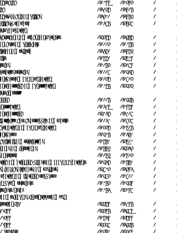
Finally, X is a vector of other factors influencing the probability of childbirth and job retention. Control variables, the vector X, are wife’s age, wife’s education, husband’s annual income, wife’s industry, wife’s occupation, and residency prefecture. Tables 1 to 3 show descriptive statistics.

Wife’s education has four categories: junior high school, high school, junior/technical college, and college/graduate. Higher education could negatively influence childbirth and positively influence job retention because of the higher opportunity cost for working women.

Husband’s income is also an important determinant of child-bearing decisions and the wife’s decision to remain employed.

We also consider that conditions for women vary among industries and occupations and control for its effect. Relevant information for January 2006 is taken from the 2007 survey and for January 2001 from the 2002 survey. Residence area (prefecture) also should be controlled because labor market conditions or availability of childcare facilities could vary widely by area.

Making Tokyo the reference category, we employed 46 area dummy variables; however, results are excluded in this paper for brevity.

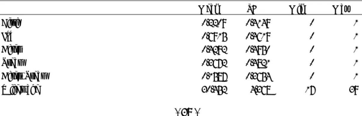
Table 1 Descriptive statistics (Number of children aged one to14 = 0)

Mean SD Min Max

Birth 0.2209 0.4149 0 1

Job 0.6915 0.4619 0 1

After 0.4292 0.4950 0 1

Treat 0.3672 0.4821 0 1

After*Treat 0.1587 0.3654 0 1

Wife's age 30.452 4.368 17 39

(8)

- 40 -

Wife's education

Junior high 0.0198 0.1393 0 1

High 0.4027 0.4905 0 1

Junior/Technical college 0.4310 0.4952 0 1

College/Graduate 0.1465 0.3536 0 1

Wife's occupation

Professional and technical workers 0.2377 0.4257 0 1

Managers and officials 0.0003 0.0175 0 1

Clerical and related 0.4470 0.4972 0 1

Sales 0.0870 0.2819 0 1

Service 0.1053 0.3069 0 1

Protective service 0.0006 0.0247 0 1

Transport and communication 0.0037 0.0603 0 1

Manufacturing and construction 0.1185 0.3232 0 1

Wife's industry

Mining 0.0005 0.0225 0 1

Construction 0.0408 0.1979 0 1

Manufacturing 0.2147 0.4106 0 1

Electricity, gas, heat supply, and water 0.0041 0.0636 0 1

Information and communication 0.0337 0.1805 0 1

Transport 0.0215 0.1451 0 1

Wholesale and retail trade 0.1751 0.3801 0 1

Finance and insurance 0.0583 0.2343 0 1

Real estate 0.0082 0.0903 0 1

Eating and drinking places and accommodations 0.0247 0.1551 0 1

Medical, health care, and welfare 0.2613 0.4394 0 1

Education and learning support 0.0263 0.1600 0 1

Compound services 0.0153 0.1229 0 1

Services, n.e.c. 0.1154 0.3196 0 1

Husband's income (in ten thousand yen)

Less than 250 0.2279 0.4195 0 1

250-299 0.2395 0.4268 0 1

300-399 0.1749 0.3799 0 1

400-599 0.2326 0.4225 0 1

600 or over 0.1251 0.3308 0 1

N=9850

Prefecture is not shown here.

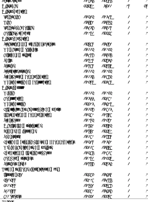
Table 2 Descriptive statistics (Number of children aged one to 14 = 1)

Mean SD Min Max

Birth 0.1434 0.3505 0 1

Job 0.8269 0.3783 0 1

After 0.4789 0.4996 0 1

Treat 0.3639 0.4812 0 1

(9)

- 41 -

After*Treat 0.1745 0.3795 0 1

Wife's age 32.281 4.300 19 39

Wife's education

Junior high 0.0202 0.1408 0 1

High 0.4571 0.4982 0 1

Junior/Tech. college 0.4047 0.4909 0 1

Wife's occupation

Sales 0.0819 0.2743 0 1

Service 0.0969 0.2958 0 1

Wife's industry

Mining 0.0002 0.0132 0 1

Transport 0.0192 0.1371 0 1

Real estate 0.0061 0.0779 0 1

Services, n.e.c. 0.0957 0.2942 0 1

less than 250 0.2363 0.4249 0 1

250-299 0.2116 0.4085 0 1

300-399 0.1830 0.3867 0 1

400-599 0.2361 0.4247 0 1

600 or over 0.1330 0.3396 0 1

N=5738

Table 3 Descriptive statistics (Number of children aged one to14 >1)

Mean SD Min Max

Birth 0.0367 0.1881 0 1

Job 0.9401 0.2373 0 1

(10)

- 42 -

After 0.4728 0.4993 0 1

Treat 0.3013 0.4588 0 1

After*Treat 0.1475 0.3547 0 1

Wife's age 34.700 3.320 21 39

# of children aged 1-14 2.2723 0.4960 2 5

Wife's education

Junior high 0.0221 0.1471 0 1

High 0.5233 0.4995 0 1

Junior/Tech. college 0.3841 0.4864 0 1

Wife's occupation

Sales 0.0831 0.2761 0 1

Service 0.0928 0.2902 0 1

Wife's industry

Mining 0.0010 0.0321 0 1

Transport 0.0203 0.1410 0 1

Real estate 0.0053 0.0726 0 1

Services, n.e.c. 0.0849 0.2788 0 1

less than 250 0.2539 0.4353 0 1

250-299 0.1755 0.3804 0 1

300-399 0.1606 0.3672 0 1

400-599 0.2533 0.4349 0 1

600 or over 0.1567 0.3636 0 1

N=7734

(11)

- 43 - 5.2 Estimation results

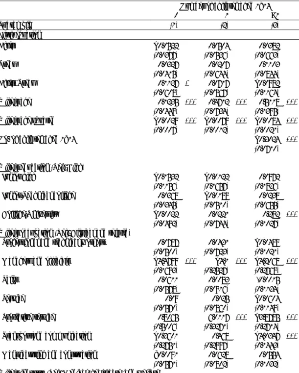
Table 4 reports the results of bivariate probit estimation. We first refer to the effect on childbirth.

In subsample (1), the coefficient of After*Treat shows a positive and significant effect, although at the 10% significance level. In subsamples (2) and (3), no effect for the Act is found.

We find that the Act has a positive effect on first births, but the significance level is low.

There may be three reasons for this result. First, sufficient time had not passed since the Act’s implementation. Large firms began to support employees’ child-bearing and rearing when the Act was implemented, but it is reasonable to assume that its influence on behavior was not immediate. In addition, the Act provides only an intangible incentive—a certification of good practice for compliant firms—but no punishment for non-compliant firms. This weak enforcement might undermine the effect of the Act. Finally, Japan already had enacted legislation related to children and work retention, such as a child allowances and paid maternity leave. The Act did not introduce new provisions in this area, and thus its impact on the estimation equation for births might be weak. Nevertheless, our results demonstrate that the Act has had a positive effect on decisions to have children, which indicates the policy is effective in reversing declining birthrates.

We also find no effect of the Act on second and subsequent births. One possible reason for this result is that working women rearing children, in subsamples (2) and (3), have already balanced work and family; Therefore, the Act may not have influenced their decisions.

Concerning results for other variables, Wife’s age shows a diminishing positive effect.

The number of children aged from one to 14, only in subsample (3), has a statistically significant, negative effect on childbirth. Wife’s education, the effect of college/university, has positive significance only in subsample (3) and is thus totally ambiguous. Certain industries show a negative effect on childbirth compared to the medical, healthcare, and welfare industries.

With respect to the influence of occupation, the variable managers and officials has a negative effect on childbirth compared to clerical and related workers. Husband’s high annual income may decrease the probability of childbirth because of the interaction between parents’ demand for quality and quantity of children, as suggested by Becker (1960, 1981).

Next, we note the effect on job retention, shown in the lower part of Table 4. In all subsamples, the coefficients of After*Treat show no significant effect. After has a significantly positive effect on job retention, reflecting that women being part of the workforce is a sustained trend. Treat shows an unclear effect. In consequence, we find no evidence that the Act influenced women’s decisions to remain employed. For second and subsequent births, as previously explained, women perhaps have already resolved the conflict between work and family. The reason for effects on first births is discussed later.

(12)

- 44 -

Turning to results of other variables related to job retention, wife’s age, the number of children aged from one to 14, and wife’s education all show ambiguous effects. For the effect of occupation, female managers and officials are more likely to continue to work; this probably explains the negative effect on childbirth. Moreover, most industries show a negative effect on job continuance compared to the medical, healthcare, and welfare industries. The effect of the husband’s annual income on wives’ job retention is slightly unclear.

Table 4 Estimation results

Number of children aged 1–14

0 1 >1

Subsample (1) (2) (3)

Birth equation

After −0.0522 0.0504 0.0382

(0.0377) (0.0536) (0.0663)

Treat 0.0327 0.0207 0.1103

(0.0415) (0.0644) (0.0844)

After*Treat 0.1127 * 0.0717 −0.0982

(0.0608) (0.0867) (0.1164)

Wife’s age 0.1235 *** 0.4712 *** 0.5118 ***

(0.0449) (0.0734) (0.1395)

Wife’s age squared −0.0029 *** −0.0079 *** −0.0084 ***

(0.0007) (0.0012) (0.0021)

No. of children aged 1–14 −0.3024 ***

(0.0710) Wife’s education (Ref: High)

Junior high −0.1532 −0.0122 0.0972

(0.1156) (0.1657) (0.1836)

Junior/Technical college 0.0368 −0.0189 0.0238

(0.0345) (0.0510) (0.0655)

College/University −0.0022 0.0221 0.282 ***

(0.0492) (0.0744) (0.1027) Wife’s occupation (Ref: Clerical and related)

Professional and technical workers 0.0787 0.0431 −0.0489 (0.0500) (0.0723) (0.1021)

Managers and officials −4.4799 *** −4.1 *** −4.2068 ***

(0.1693) (0.2527) (0.2768)

Sales 0.0611 0.0083 -0.0015

(0.0578) (0.0916) (0.1134)

Service 0.09 0.025 −0.0604

(0.0570) (0.0860) (0.1149)

Protective service 0.8065 6.0117 *** −3.8785 ***

(0.5006) (0.3271) (0.2714)

Transport and communication −0.3601 0.468 −4.0347 ***

(0.2751) (0.2997) (0.1443)

Manufacturing and construction –0.0091 0.0628 0.0554

(0.0571) (0.0802) (0.1032) Wife’s industry (Ref: Medical, healthcare, and welfare)

(13)

- 45 -

Mining −4.9267 *** −3.3875 *** 0.3867

(0.1294) (0.2664) (0.5554)

Construction −0.1445 * −0.1767 −0.3356 **

(0.0869) (0.1223) (0.1528)

Manufacturing −0.1521 ** −0.1777 ** −0.3112 **

(0.0602) (0.0888) (0.1251) Electricity, gas, heat supply, and water −0.0573 −0.7852 −4.5206 ***

(0.2248) (0.4799) (0.1400) Information and communication −0.3304 *** −0.1309 −0.3526 (0.0938) (0.1376) (0.2749)

Transport −0.1196 −0.2076 −0.8248 **

(0.1133) (0.1789) (0.3751)

Wholesale and retail trade −0.0783 −0.2098 ** −0.1577

(0.0594) (0.0891) (0.1208)

Finance and insurance −0.1091 −0.191 −0.118

(0.0790) (0.1169) (0.1553)

Real estate 0.2162 −0.6659 * −0.3399

(0.1542) (0.3424) (0.4283) Eating and drinking places and accommodations −0.0248 −0.1838 −0.1905 (0.0990) (0.1686) (0.1915)

Education and learning support 0.0248 0.1617 0.0251

(0.0936) (0.1262) (0.2107)

Compound services −0.0799 −0.0639 −0.0611

(0.1265) (0.1688) (0.1916)

Service, n.e.c. −0.1541 *** −0.1931 ** −0.0152

(0.0578) (0.0894) (0.1149) Husband’s income (Ref: less than 250)

250–299 0.0569 0.0195 0.0403

(0.0415) (0.0618) (0.0801)

300–399 0.06 0.0405 −0.0449

(0.0462) (0.0652) (0.0855)

400–599 −0.0188 −0.0258 0.0201

(0.0454) (0.0655) (0.0807)

600 or more −0.367 *** −0.2014 *** −0.2826 ***

(0.0560) (0.0765) (0.1018)

Constant −1.7824 *** −7.8489 *** −8.5142 ***

(0.6791) (1.1556) (2.3200)

Job equation

After 0.3126 *** 0.1814 *** 0.2441 ***

(0.0360) (0.0532) (0.0589)

Treat 0.0714 * −0.0757 −0.1368 **

(0.0392) (0.0593) (0.0688)

After*Treat −0.0848 0.1357 0.096

(0.0587) (0.0863) (0.1017)

Wife’s age 0.0321 0.0445 0.2576 **

(0.0420) (0.0648) (0.1056)

Wife’s age squared 0.0007 0.0006 −0.003 *

(0.0007) (0.0010) (0.0016)

No. of children aged 1–14 0.0234

(0.0517) Wife’s education (Ref: High)

Junior high −0.0690 −0.0332 −0.3284 **

(0.1035) (0.1535) (0.1274)

Junior/Tech. college 0.0337 −0.0416 0.0248

(14)

- 46 -

(0.0330) (0.0497) (0.0559)

College/University 0.1710 *** 0.0769 0.1323

(0.0475) (0.0752) (0.1016) Wife’s occupation (Ref: Clerical and related)

Professional and technical workers 0.0753 0.0052 −0.086 (0.0480) (0.0714) (0.0915)

Managers and officials −0.2834 3.9022 *** 4.1867 ***

(0.7363) (0.2503) (0.2498)

Sales −0.0455 −0.1357 * −0.1271

(0.0538) (0.0802) (0.0905)

Service −0.0139 0.0255 −0.0771

(0.0545) (0.0872) (0.1053)

Protective service 0.2198 −5.556 *** 4.0188 ***

(0.5289) (0.3225) (0.2542)

Transport and communication −0.1947 −0.5357 * −0.5348

(0.2425) (0.2799) (0.3565)

Manufacturing and construction 0.0368 0.0852 −0.0673

(0.0544) (0.0778) (0.0816) Wife’s industry (Ref: Medical, healthcare, and welfare)

Mining −0.3698 2.9983 *** 4.0915 ***

(0.5249) (0.2696) (0.1966)

Construction −0.0103 −0.1942 −0.0251

(0.0825) (0.1196) (0.1313)

Manufacturing 0.1496 ** −0.1711 ** −0.1604

(0.0587) (0.0870) (0.1058) Electricity, gas, heat supply, and water 0.3515 −0.0785 0.1812 (0.2243) (0.3226) (0.4497)

Information and communication −0.0183 −0.1607 −0.0434

(0.0847) (0.1380) (0.2171)

Transport 0.0792 −0.2712 * 0.2022

(0.1069) (0.1574) (0.2066) Wholesale and retail trade −0.1269 ** −0.3052 *** −0.181 *

(0.0563) (0.0844) (0.1076)

Finance and insurance −0.124 * −0.2952 *** −0.4051 ***

(0.0734) (0.1106) (0.1294)

Real estate −0.5228 *** −0.2797 −0.1934

(0.1507) (0.2586) (0.3011) Eating and drinking places and accommodations −0.3768 *** −0.3431 ** −0.226 (0.0932) (0.1490) (0.1587) Education and learning support −0.3415 *** −0.5802 *** −0.7885 ***

(0.0877) (0.1215) (0.1619)

Compound services 0.6506 *** 0.5575 ** −0.0716

(0.1451) (0.2181) (0.1937)

Service, n.e.c. −0.0711 −0.1287 −0.1339

(0.0552) (0.0888) (0.1100) Husband’s income (Ref: less than 250)

250–299 −0.0867 ** −0.03 −0.0925

(0.0410) (0.0621) (0.0750)

300–399 −0.2366 *** −0.0971 −0.185 **

(0.0450) (0.0658) (0.0761)

400–599 −0.3161 *** −0.1401 ** −0.1589 **

(0.0440) (0.0647) (0.0715)

600 or more 0.1359 *** 0.0509 −0.1206

(0.0518) (0.0758) (0.0770)

(15)

- 47 -

Constant −0.8737 −1.1419 −3.6535 **

(0.6374) (1.0078) (1.7336)

ρ −0.4712 *** −0.0534 * −0.2731 ***

Log likelihood −10100 −4630 −2750

N 9850 5738 7734

*** p<0.01, ** p<0.05, * p<0.1

Robust standard errors are in parenthesis.

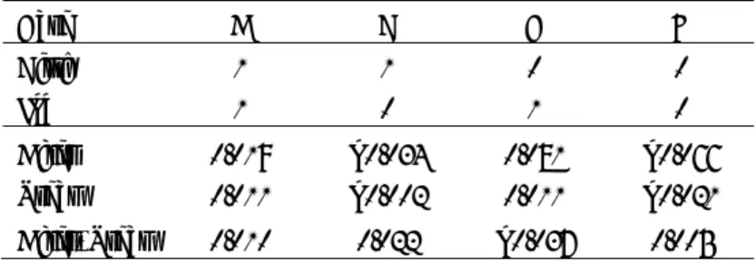
5.3 Marginal effect of the Act

Here, we discuss the Act’s marginal effect on childbirth and women’s job retention using subsample (1)—that is, the sample involving first births.

Table 5 shows the marginal effects of the Act in four cases. Case A, the probability of continuing to work after giving birth, shows about a 1% increase. Case B, the probability of giving birth and quitting work, shows about a 2.2% increase. The probability of Case B is about double that of Case A. Case C, the probability of women continuing to work without having children, shows a 3.7% decrease.

The Act certainly increased the number of women who continued to work after having children (Case A). However, it also increases the number of women who quit their jobs when they gave birth (Case B). These results imply two possibilities. First, women working for large firms may have been able to resolve conflicts between child-bearing and work more easily than before the Act. However, because “the problem of children on a waiting list for a daycare center” persists, especially in urban areas, women still face difficulty balancing child-bearing and work. Second, as a recent Japanese Time-Use Survey shows, husbands have not increased their contributions toward childcare and housework. In consequence, women have to choose either giving birth or working continuously. The Act boosts child-bearing by reducing the number of women in Case C. However, it increases numbers in Cases A and B, offsetting the Act’s effect on women’s job retention.

Table 5 Marginal effects of the Act for subsample (1)

Case A B C D

Birth 1 1 0 0

Job 1 0 1 0

After 0.019 −0.034 0.081 −0.066

Treat 0.011 −0.002 0.011 −0.021

After*Treat 0.010 0.022 −0.037 0.005

(16)

- 48 -

6 Conclusion

The Japanese government has recently changed its policy direction for measures intended to reverse the nation’s declining birthrate and now focuses on the role of firms. As part of this new policy direction, the Act on Advancement of Measures to Support Raising Next-Generation Children took effect in 2005. The Act requires large firms to support their employees in bearing and rearing children.

Thus, this study has investigated the act’s effect on childbirth and on women’s job retention. Our DID estimation, using the quasi-experimental condition, demonstrates that the policy has a positive effect of about 1% on the joint probability of first births and women’s job retention. This indicates that the Act can reduce the opportunity cost of having children for working women and that firms play important roles in improving Japan’s birthrate. However, the Act also increases the probability that women will quit their jobs after giving birth. That outcome may be tied to the shortage of childcare facilities and to husbands’ static contributions to household chores. Although the Act shows unexpected effects, the change in policy direction is partially successful in encouraging employees to have children.

Acknowledgements

The Employment Status Survey is provided by The Ministry of Internal Affairs and Communications. This research is supported by Health Labour Sciences Research Grant (The Ministry of Health, Labour and Welfare).

References

Adserà A (2004) Changing fertility rates in developed countries. The impact of labor market institutions. J Popul Econ 17:17–43.

Averett AL, Whittington LA (2001) Does maternity leave induce birth? South Econ J 68(2):403–417.

Azmat G, González L (2010) Targeting fertility and female participation through the income tax.

Labour Econ 17(3):487–502.

Baum CL (2003) The effect of state maternity leave legislation and the 1993 Family and Medical Leave Act on employment and wages. Labour Econ 10(6):573–596.

(17)

- 49 -

Becker GS (1960) An economic analysis of fertility in Demographic and Economic Change in Developed Countries, Universities-National Bureau Conference Series 1. Princeton Univ.

Press:209–240.

Becker GS (1981) A treatise on the family. Harvard Univ. Press.

Buttner T, Lutz W (1990) Estimating fertility responses to policy measures in the German Democratic Republic. Popul and Dev Rev 16(3):539–555.

Del Boca D (2002) The effect of child care and part time opportunities on participation and fertility decisions in Italy. J Popul Econ 15:549–573.

Gupta ND, Smith N, Verner M (2008) The impact of Nordic countries’ family friendly policies on employment, wages, and children. Rev Econ Househ 6:65–89

Haah P, Wrohlich K (2011) Can child care policy encourage employment and fertility?:

Evidence from a structural model. Labour Econ 18(4):498–512.

Higuchi Y (1994) Ikuji Kyugyo Seido no Jissho Bunseki (An empirical analysis on the parental leave). In Shakai Hosho Kenkyujo (eds) Gendai Kazoku to Shakai Hosho: Kekkon, Shussho, Ikuji (Contemporary Family and Social Security: Marriage, Childbirth, and Childcare) University of Tokyo Press, pp 181–204.

Japanese Cabinet Office (2011) White paper on birthrate-declining society 2011.

Kalwij A (2010) The impact of family policy expenditure on fertility in western Europe.

Demogr 47(2):503–519.

Lundin D, Mörk E, Öckert B (2008) How far can reduced childcare prices push female labour supply? Labour Econ 15(4):647–659.

McNown R, Ridao-Cano C (2004) The effect of child benefit policies on fertility and female labor force participation in Canada. Rev Econ Househ 2:237–254.

Morita Y (2005) Ikuji Kyugyo Ho no Kiseiteki Sokumen: Rodo Juyo heno Eikyo ni Kansuru Shiron(The Child-Care Leave Law and the demand for female labor), Nihon Rodo Kenkyu Zasshi 536:123–136.

Morita Y, Kaneko Y (1998) Ikuji Kyugyo Seido no Fukyu to Josei Koyosha no Kinzoku Nensu (The effect of the child care leave on women in the workforce). Nihon Rodo Kenkyu Zasshi 459:50–62.

Ruhm C J (1998) The economic consequences of parental leave mandates: lessons from Europe.

Q J Econ 113(1):285–317.

Sánchez-Mangas R, Sánchez-Marcos V (2008) Balancing family and work: the effect of cash benefits for working mothers. Labour Econ 15(6):1127–1142.

Schellekens J (2009) Family allowances and fertility: Socioeconomic differences. Demogr 46(3):451–468.

(18)

- 50 -

Tanaka R, Kouno T (2009) Shussan Ikuji Ichijikin ha Shusshouritu wo Hikiageruka: Kenko Hoken Kumiai Panel Data wo Mochiita Jisshou Bunseki (Do childbirth allowances matter for fertility?: Evidence from the Japanese health insurance data) Nihon Keizai Kenkyu 61:94–108.

Waldfogel J, Higushi Y, Abe M (1999) Family leace policies and women’s retention after childbirth: evidence from the United States, Britain and Japan. J Popul Econ 12(4): 523–545.

Willis R (1973) A new approach to the economic theory of fertility behavior. J Polit Econ 81(2):S14–S64.

Whittington LA, Alm J, Peters HE (1990) Fertility and the personal exemption: Implicit pronatalist policy in the United States. Am Econ Rev 80(3):545–556.

Yoshida H, Mizuochi M (2005) Ikuji Shigen no Riyo Kanosei ga Shusshouryoku oyobi Josei no Shugyo ni Ataeru Eikyo (The effect of childcare resources on fertility and women’s labor supply) Nihon Keizai Kenkyu 51:76–95.

Zhang J, Quan J, Van Meerbergen P (1994) The effect of tax-transfer policies on fertility in Canada, 1921–88. J Hum Resour 29(1):181–201.