Simulated Annealing with Advanced Adaptive Neighborhood
Mitsunori MIKI
†, Tomoyuki HIROYASU
†, Keiko ONO
†††
Department of Knowledge Engineering,
††
Graduate Student, Doshisha University
Kyo-tanabe, Kyoto, 610-0321, JAPAN Email: [email protected]
1 Introduction
It was Kirkpatrick et al. who first proposed simulated annealing, SA, as a method for solving combinatorial optimization problems[1]. It is reported that SA is very useful for several types of combinatorial optimization prob- lems[2]. The advantages and the disadvantages of SA are well summarized in [3]. The most remarkable disadvantages are that it needs a lot of time to find the optimum solution and it is very difficult to determine the proper cooling schedule. To determine the proper cooling schedule, many preparatory trials are needed. When the cooling schedule is not proper, the guarantee of finding optimum solution is lost.
There are two approaches to shorten the calculation time in SA. One is determining the cooling schedule properly.
SA with the proper cooling schedule can provide an optimum solution quickly. This approach is well reported by Ingber[3]. The other approach is to choose a proper neighborhood. For discrete or combinatorial optimization problems, the neighborhood structure is uniquely determined by the generation method of a new solution from the current one and it is difficult to control. However, the neighborhood structure for continuous optimization problems is very simple, and it is easily controlled by the neighborhood range, or the scaling parameter of the search step.
In this paper, we propose a new method for controlling the neighborhood range in continuous optimization prob- lems to obtain good solutions in shorter annealing steps. The Corana’s method[4] which controls the neighborhood range is very useful since the method automatically determines the neighborhood range, but the performance of the method in terms of the search ability has not been clear. We investigate the performance of the Corana’s method, and show the necessity of introducing a new adaptive method which controls the neighborhood range and also provides high searching performance.
2 Adaptive Neighborhood with the Acceptance Rate is 0.5
2.1 Corana’s Method
Corana[4] proposed an adaptive method of SA for continuous optimization problems. The neighborhood range is adjusted to keep the acceptance rate of 0.5 in this method. The generation of a new solution is carried out with the following equation, where x
iis the current solution, x
iis the next candidate solution, r is a uniform random number with the interval [-1, 1] and m is the neighborhood range.
x
i= x
i+ rm (1)
The neighborhood range m is varied according to the acceptance rate p, as follows.
m
= m × g(p) g(p) = 1 + c
p−pp 12
, if p > p
1g(p) =
1 + c
p2p−p2
−1, if p < p
2g(p) = 1, otherwise
p
1= 0.6, p
2= 0.4
(2)
where c is a scaling parameter. The acceptance rate p can be calculated from the number of acceptance n within the period N where the neighborhood range is constant, as follows.
p = n/N (3)
2.2 Problem in the Corana’s Method
The design of neighborhood structure becomes very easy with the application of the Corana’s method for continuous optimization problems solved by SA. However, the validity of the fixed acceptance rate of 0.5 is not clear.
Corana did not show the evidence of the validity. Miki et al.[5] found that the the performance of the Corana’s method is not better than the SA with the optimum fixed neighborhood range. Therefore, the validity of the goal acceptance rate of 0.5 is unreliable.
To find the weak point of the Corana’s method, the detailed analysis of the result obtained by the method is conducted. For the Rastrigin function, which is one of the standard test function for many heuristic search algorithms, the neighborhood range and the value of the energy function are shown in Fig. 1. One can see that the neighborhood range is decreased as the annealing steps increase, while the energy is not deccreased. From the simple consideration about the Rastrigin function, the maximum distance of the local optimum region is 1.0, and the neighborhood range should be larger than this value to escape a local minimum. However, the neighborhood range shown in Fig. 1 is decreased below 1.0 at the very early stage of the search process. Therefore, the move of the solution is trapped in a local minimum and the history of the energy shows such situation since the global minimum has the energy of 0.
The reason why the Corana’s method yields this situation is as follows. When the solution is at a local optimum and the neighborhood range is smaller than the distance of the local optimum region, the next move of the current solution always gives a higher energy. Then, the acceptance rate is decreased and the neighborhood range is decreased accoding to this small acceptance rate, as shown in Eq. (2). This means that the solution can not escape from the local minimum further more. From this consideration, it can be concluded that the Corana’s method acceralate the trapping of the solution into a local minimum.
Figure 1: Histories of energy and neighborhood rane(Rastrigin)
3 New Approach to Adaptive Neighborhood
3.1 Improvement over the Corana’s method
The goal acceptance rate of 0.5 in the Corana’s method is found to give poor performance in the search ability of SA since the neighborhood range becomes too small. Therefore, the goal acceptance rate which is smaller than 0.5 is considered here to increase the neighborhood range.
Firstly, the values of p
1and p
2in Eq. (2) are modified to maintain the acceptance rates of 0.3, 0.1, and 0.01. For
example, p
1= 0.05 and p
2= 0.15 for the goal acceptance rate of 0.1. At the beginning of the annealing steps, the
temperature is very high and such low acceptance rate cannot be realized. Therefore, the goal acceptance rate is 0.5
at this stage, and then the goal acceptance rate is changed to the lower value.
Figure 2 shows the history of the acceptance rate during the annealing for the goal acceptance rate of 0.1. The goal acceptance rate is 0.5 at the beginning and it is changed to 0.1 at the annealing step of 1.0 × 10
5. However, it is seen that the acceptance rate becomes around 0.27 and it is not decreased to 0.1. The neighborhood range in this case is shown in Fig. 3. The neighborhood range is increased slightly at the annealing steps of 1.0 × 10
5, where the goal acceptance rate is changed to 0.1 from 0.5, but the neighborhood range is still below 1.0. In this situation, it is impossible for a solution to escape from a local minimum. From this result, it can be concluded that the magnification factor of the neighborhood range is too small in this case, that is, it is problem-dependent and it should be adaptive to problems.
Figure 2: History of acceptance probability(Rastrigin)
Figure 3: History of neighborhood range(Rastrigin)
3.2 Design of New Adaptive Neighborhood
In section 3.1, the improvement over the Corana’s method which yields the lower acceptance rate failed. To realize a low acceptance rate, the neighborhood range should be large enough to escape local minima. The maximum magnification factor of the neighborhood range is fixed to a constant value, (3.0), in the Corana’s method. In many cases, this value is not enough to escape from local minima. However, the appropriate value for the maximum magnification factor is not clear since it is problem-dependent. Therefore, a new adaptive mechanism for the adaptive neighborhood is proposed here. The new algorithm is called SA/AAN, Simulated Annealing with Advanced Adaptive Neighborhood, and this algorithm provides a low acceptance rate such as 0.1.
The neighborhood range is determined by Eq. (4) where the magnification factor of the range, g(p), is the function of H
0, and H
0is increased or decreased recursively according to the actual acceptance rate, as shown in Eq.
(6). That is, the magnification factor can be increased to a very large value when the acceptance rate is larger than the goal acceptance rate.
m
= m × g(p)
g(p) = H
0(p
), if p > p
1g(p) = 0.5, if p < p
2g(p) = 1.0, otherwise
(4)
H
0= H
0× H
1,
(initial value: H
0= 2.0)
H
1= 2.0, if p
> p
1H
1= 0.5, if p
< p
2H
1= 1.0, otherwise
(5)
where p is calculated by Eq. (3), and p’ is calculated by Eq. (6), and p
1and p
2are the upper and lower bounds of the goal acceptance probability.
p
= l/L (6)
At the beginning of the annealing process, however, a low acceptance rate cannot be realized since the temperature is very high. Therefore, the goal acceptance rate is set to 0.5 at the beginning, and after that the neighborhood range is fixed. Then, the acceptance rate is decreased naturally since the solution moves to a better location. The proposed algorithm is applied when the acceptance rate is decreased to the goal acceptance rate.
4 Optimization problems
To examine the search performance of the proposed method, three standard test functions are used. Those are the Rastrigin function[6] shown in Eq. (7), the Griewangk function[7] shown in Eq. (8), and the Rosenbrock function[7]
shown in Eq. (9). The number of design variables is two for all functions. The optimum solutions are located at the origin for the Rastrigin and Griewangk functions, and the function values are both 0, and the optimum solution is located at (1,1) for the Rosenbrock function, and its function value is also 0.
f
R(x) = (N × 10) +
Ni=1
x
2i− 10 cos(2πx
i)
(7) domain : −5.12 < x
i≤ 5.12,
optimum solution : (x
1, x
2) = (0, 0), optimum value : f = 0
f
G(x) = 1 +
N i=1x
2i4000
−
Ni=1
cos
x
i√ i
(8) domain : −600 < x
i≤ 600,
optimum solution : (x
1, x
2) = (0, 0), optimum value : f = 0
f
Ro(x) = 100(x
2− x
21)
2+ (1 − x
1)
2(9) domain : −2 < x
i≤ 2,
optimum solution : (x
1, x
2) = (1, 1), optimum value : f = 0
The parameters used for the numerical experiments for these three test functions are shown in Table 1, where the detailed method of the determination of these parameters are shown in [5].
5 Experimental Results and Discussions
5.1 Change in the acceptance rate
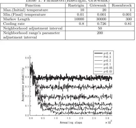
The history of the acceptance probability is shown in Fig. 4, where the abscissa is the number of annealing steps
and the ordinate is the acceptance probability averaged over 1000 annealing steps. From this figure, the acceptance
probabilities are maintained to the prescribed goal values, and the proposed method can provide a small constant
acceptance probability.
Table 1: Parameter(Rastrigin, Griewank)
Function Rastrigin Griewank Rosenbrock
Max.(Initial) temperature 10 20 1
Min.(Final) temperature 0.01 0.001 0.001
Markov Length 10000 30000 300
Cooling rate 0.8 0.726 0.81
Neighborhood adjustment interval 50
Neighborhood range’s parameter 200
adjustment interval
Figure 4: History of acceptance probability(Rastrigin)
5.2 Performance of SA/AAN
The energy values of the optimum solutions obtained for three test functions are shown in Fig. 5 for various constant acceptance probabilities. The energy values are the medians for 10 trials each, where the median gives more appropriate evaluation for the final energy value than the average since the range of the final energy is very large.
From Fig. 5, the Corana’s method which maintains the acceptance probability to 0.5 does not provide good performance, and the optimum goal acceptance probability is found to be very small such as 0.05 through 0.2.
Figure 5: Energy of optimum value
5.3 Effectiveness of SA/AAN
The reason why the proposed method provides good results is clearly found from Fig. 6, where the history of
the energy of the Rastrigin function is shown as the function of the annealing steps. From this figure, it is found
that the solution obatined by the Corana’s method is trapped in a local optimum, while the solution obtained by
the proposed method goes to the global optimum.
This difference stems from the difference of the change of the neighborhood ranges. Figure 7 shows the histories of the neighborhood ranges for the Corana’s method and the proposed method. The neighborhood range in the Corana’s method decreses quickly and becomes less than 1.0 at the early stage of the search process, but the neighborhood range in the proposed method decreases gradually and it sometimes increases on a large scale and this helps the solution to escape from local optima. Thus the new adaptive mechanism of the neighborhood range is found to be very effective to continuous optimization problems.
Figure 6: History of energy(Rastrigin)
'
0GKIJDQTJQQFTCPIG
#PPGCNKPIUVGRU
5###0
%QTCPC