Faster Rotation-Based Gauss Sieve for Solving the SVP on General Ideal Lattices

PAPER

Faster Rotation-Based Gauss Sieve for Solving the SVP on General Ideal Lattices

Shintaro NARISADA^†a), Hiroki OKADA^†, Kazuhide FUKUSHIMA^†,andShinsaku KIYOMOTO^†,Members

SUMMARY The hardness in solving the shortest vector problem (SVP) is a fundamental assumption for the security of lattice-based cryptographic algorithms. In 2010, Micciancio and Voulgaris proposed an algorithm named the Gauss Sieve, which is a fast and heuristic algorithm for solv- ing the SVP. Schneider presented another algorithm named the Ideal Gauss Sieve in 2011, which is applicable to a special class of lattices, called ideal lattices. The Ideal Gauss Sieve speeds up the Gauss Sieve by using some properties of the ideal lattices. However, the algorithm is applicable only if the dimension of the ideal latticenis a power of two orn+1 is a prime.

Ishiguro et al. proposed an extension to the Ideal Gauss Sieve algorithm in 2014, which is applicable only if the prime factor ofnis 2 or 3. In this paper, we first generalize the dimensions that can be applied to the ideal lattice properties to when the prime factor ofnis derived from 2, porq for two primespandq. To the best of our knowledge, no algorithm using ideal lattice properties has been proposed so far with dimensions such as:

20, 44, 80, 84, and 92. Then we present an algorithm that speeds up the Gauss Sieve for these dimensions. Our experiments show that our proposed algorithm is 10 times faster than the original Gauss Sieve in solving an 80- dimensional SVP problem. Moreover, we propose a rotation-based Gauss Sieve that is approximately 1.5 times faster than the Ideal Gauss Sieve.

key words: shortest vector problem, Gauss Sieve, ideal lattice, generaliza- tion

1. Introduction

Lattice-based cryptography has attracted interest as a fun- damental theory for designing candidates for quantum- resistant cryptographic algorithms. The security of lattice- based cryptographic algorithms is based on the hardness in solving the shortest vector problem (SVP). In 1998, Ajtai[1]

proved that the SVP is a class of NP-hard problems. He in- troduced the concept of the lattice-based cryptography as well. A deterministic algorithm for solving the SVP called Enumeration was proposed[2]in 1981, and Ajtai et al. pre- sented a probabilistic algorithm called Sieving[3]in 2001, respectively. Enumeration and Sieving are the two major algorithms for solving the SVP. Various sieving algorithms have been proposed and they have become the mainstream of algorithms for solving the SVP. In 2010, Micciancio and Voulgaris[4]proposed the Gauss Sieve (GS), which heuris- tically solves the SVP by recursively collecting shorter vec- tors. The GS was experimentally faster than the ordinary sieving algorithms and it was the first sieving algorithm to be competitive with the enumeration algorithm with regard to its computational cost. Ducas[5]proposed the SubSieve

Manuscript received March 16, 2020.

Manuscript revised July 1, 2020.

†The authors are with KDDI Research, Inc., Fujimino-shi, 356- 8502 Japan.

a) E-mail: [email protected] DOI: 10.1587/transfun.2020CIP0014

algorithm in 2018, which can reduce a few lattice dimen- sions by applying a technique of lattice orthogonalization.

Albrecht et al. [6]proposed a new sieving implementation calledg6k. It contains the existing sieving algorithms, and it includes some heuristic techniques for speeding-up the siev- ing procedure, such as optimization of the lattice basis up- dating process. g6k can solve the SVP with higher dimen- sions.

A special lattice named the Ideal Lattice contributes to reduce the computation time of cryptosystems [7], [8].

Schneider [9] presented that some types of ideal lattices are useful for reducing the computational time of the GS.

He characterized these ideal lattices as theAnti-cyclic lat- tice and the Prime cyclotomic lattice. Then, he proposed the Ideal Gauss Sieve (IGS) by utilizing the properties of their rotation structures. The IGS is faster than the GS if the lattice dimension nis 2^a or p−1 for an odd prime p.

Similar IGS techniques[10]enable speeding up the LLL al- gorithm [11], which is a lattice basis reduction algorithm.

In[12], Ishiguro et al. considered a special case of ideal lat- tices called atrinomial lattice. They claimed that the rota- tion property of the trinomial lattice could speed up the GS only ifnis 2^a3^b, in addition to the Schneider’s result of 2^a orp−1. However, no algorithm that utilizes the ideal lattice structure has been proposed in order to reduce the computa- tional time needed to solve the SVP with other dimensions.

1.1 Contributions

We propose a new ideal lattice structure named thet-nomial latticeas a generalized version of the anti-cyclic lattice, the prime cyclotomic lattice, and the trinomial lattice. Then we show that the IGS can reduce the computational time by utilizing the t-nomial lattice for dimensionsn = 2^ap^b(p− 1)q^c(q−1) (a,b,c ≥ 0, and p andq are odd primes s.t.

p<q). The equation obviously fits the previous results with dimensionsn =2^a,p−1 and 2^a3^b. Moreover, we propose an algorithm named therotation-based Gauss Sieve(RGS) algorithm that leverages the rotation structure of ideal lat- tices to reduce the internal cost of the GS. Our experiments confirm that our proposed algorithm is 1.5 times faster than the IGS.

2. Definition

Anm-dimensional vector is denoted byv =(v0, . . . , vm−1).

For 0≤i≤m−1, thei-th element ofvis written asv[i]. The Copyright c2021 The Institute of Electronics, Information and Communication Engineers

Euclidean norm of a vectorvis denoted bykvk= q Pm−1

i=0 v²_i. The inner product of two vectorsu=(u0, . . . ,um−1) andv= (v₀, . . . , v_m−1) ishu,vi=Pm−1

i=0 uiv_i. A matrixBconsisting of nlinearly independentm-dimensional vectors is denoted by B=(b₀, . . . ,b_n−1)∈R^m×n. Thelatticegenerated by a basis Bis the set of the all linear combinations of the basis vector b0, . . . ,bn−1

L(B)=L(b0, . . . ,bn−1)=











n−1

X

i=0

x_ib_i

x_i∈Z









 .

We callBthe basis of the latticeL. In the following, letn= mandbi∈Zⁿ. The determinant of a lattice generated byB is det(L(B))= p

det(B^TB). We say thatnis the dimension of the lattice. λ₁(L) is the Euclidean norm of the shortest nonzero vector inL. We define the SVP as follows.

Definition 1(SVP). For a latticeL(B), compute a vector v∈ L(B)s.t. kvk=λ₁(L(B)).

We can estimate the length of the shortest vector in the n-dimensional latticeL(B) by the Gaussian heuristic, where Γ(x) is a gamma function.

λ₁(L(B))= 1

√πΓn 2+1

¹_n

det(L(B))¹ⁿ

An idealIis the subgroup of the additive group of the ring R = Z[x]/(g(x)), whereg(x) is a monic polynomial overZ. We make a polynomial v(x) = Pn−1

i=0 vixⁱ ∈ I and its coefficient vector v = (v₀, . . . , v_n−1) ∈ Z correspond.

Then, the set {v|v(x) = Pn−1

i=0 vixⁱ ∈ I}is a lattice. These lattices satisfy the above conditions and are called ideal lattices. Let the polynomial expression of a lattice vector v∈ Lbev(x), then we write arotationof the vectorv(x) as rot(v) = xv(x) modg(x). The ideal lattice is closed under the rotation operations. Namely,v∈ L ⇒rot(v)∈ L. We writeirotations asrotⁱ(v)=rot(rotⁱ⁻¹(v)) androt⁰(v)=v.

As monic polynomials, we use the cyclotomic poly- nomials that are used in the Ring-Learning with Errors (R- LWE) problem [13]. The m-th cyclotomic polynomial is defined as follows, where gcd(i,j) represents the greatest common divisor of two natural numbersi,j

Φm(x)= Y

1≤k≤m,gcd(k,m)=1

x−e^2πik/m .

For instance,Φ8(x)=x⁴+1 andΦ12(x)=x⁴−x²+1. The degree ofΦm(x) isϕ(m)[14], whereϕ(m) is Euler’s totient function.

3. Preliminaries

We describe the outline of the GS [4] and then give an overview of the IGS[9]and Ishiguro’s extension[12]. We mention the following two definitions related to lattice vec- tors before considering the GS.

Definition 2(Gauss-reduced). Two vectorsu,v∈ L(B) are

Algorithm 1:Reduction[4]

Input: u,v∈ L(B) Output: u∈ L(B)

1 if|2hu,vi|>kvk²then u←u− hu,vi

kvk²

v

2 return u

Gauss-reduced, whereu,vholdsku±vk ≥max(kuk,kvk).

The procedure in Algorithm 1 outputs the Gauss- reduced vectors of u andv; uor vis recursively replaced by the subtraction of uandv, where the vector yielded by the subtraction has a shorter norm thanuorvdoes. This re- placement is calledreduce. Algorithm 1 details thereduce process. In acollisioncase in which two vectors are linearly dependent, the algorithm always outputs a zero vector.

Pairwise-reduced is a generalization of “Gauss- reduced”, which is extended to a set of vectors.

Definition 3 (Pairwise-reduced). For a set A ⊂ L(B), A isPairwise-reduced, where all combinations of the vectors

∀u,v∈A,u,vare Gauss-reduced.

3.1 Gauss Sieve

Micciancio and Voulgaris proposed two sieving algorithms named the List Sieve and GS[4]. The GS is a practical vari- ant of the List Sieve that probabilistically solves the SVP.

Algorithm 2 is related to the GS. The GS [4] extends a pairwise-reduced set of lattice vectorsLuntil a certain num- ber of collisions occurs. WhenLcontains a sufficient num- ber of lattice vectors, the shortest vector of the lattice is in- cluded in the setLwith a certain probability. A new lattice vector vis generated by a random sampling via a sampler such as Klein’s algorithm[15]. Klein’s sampler generates a vector by computing withinO(n²). For a fresh vectorv, the GS decreases the norm of vby performing the reduce function; so thatvand all its elements ofLbecome Gauss- reduced, and L∪ {v}is Pairwise-reduced. The GS contin- ues the above procedures until the number of collisions c reachescmax. Finally, the GS outputs the shortest vector in Las a candidate of the shortest vector of the latticeL(B).

3.2 Ideal Gauss Sieve

The IGS [9] is a variant of the GS that utilizes a rota- tion structure of specific ideal lattices calledAnti-cyclic lat- tice and Prime cyclotomic lattice. The anti-cyclic lattice is a lattice generated by a binomial cyclotomic polynomial Φm(x)=xⁿ+1.

Definition 4(Anti-cyclic lattice). Then-dimensional ideal lattice of the ringR=Z[x]/Φm(x) is said to be an anti-cyclic lattice, whereΦm(x)=xⁿ+1 (n=2^a−1,m=2^a,a>0).

The prime cyclotomic lattice is the lattice generated by an (n+1)-term cyclotomic polynomial.

Algorithm 2:Gauss Sieve[4]

Input:A basisBof the latticeL(B), maximal number of collisionsc_max

Output: A candidate of the shortest vector inL(B)

1 L← {},S← {},c←0

2 whilec<c_maxdo

3 if|S|=0then v←sample fromL(B)

4 else v←S.pop()

5 v⁰←v

6 for `∈Ldo

7 v←Reduction(v,`)

8 ifkvk=0then c←c+1

9 else if v⁰,v then S.push(v)

10 else

11 for `∈Ldo

12 `<sup>0</sup>←Reduction(`,v)

13 if`<sup>0</sup>,`then

14 L←L\ {`}

15 S.push(`⁰)

16 L←L∪ {v}

17 returnthe shortest vector inL(a candidate of the shortest vector inL(B))

Definition 5(Prime cyclotomic lattice). Thendimensional ideal lattice of the ringR = Z[x]/Φm(x) is said to be the prime cyclotomic lattice, whereΦm(x)=xⁿ+xⁿ⁻¹+· · ·+1 (n=p−1,m=p,pis a prime).

For ann-dimensional vectorvand 0 ≤i ≤n−1, the rotation of the anti-cyclic latticerot(v) is

rot(v)[i]=

( −v[n−1] (i=0) v[i−1] (otherwise).

The time complexity ofrot(v) for an anti-cyclic lattice is O(1) when using a bidirectional list. v has the same Eu- clidean norm asrot(v). The rotation of the prime cyclotomic lattice is

rot(v)[i]=

( −v[n−1] (i=0) v[i−1]−v[n−1] (otherwise).

The computational complexity ofrot(v) for the prime cy- clotomic lattice is O(n). In general, the norm ofrot(v) is different from the norm ofv, and it is not larger than 2kvk.

Schneider applied these rotation formulae to implement the Reduction function, i.e., if input of GS is an ideal lattice, Reduction in Algorithm 2 can be replaced by ReduceRot function in Algorithm 3. The ReduceRot function increases the probability of reducing the norm of usincerotⁱ(v) for alli > 0 is used to reduceu in addition tov. The proba- bility Pr[ku⁰k < kuk | u⁰ = Reduction(u,rotⁱ(v))] for any i is identical to Pr[ku⁰k < kuk | u⁰ = Reduction(u,v)] if input basis is the prime cyclotomic lattice androtⁱ(v) is lin- early independent ofv, sincerotⁱ(v) for anyisatisfies that krotⁱ(v)k = kvk. Note that there exist two vectorsuandv such that Reduction(u,rotⁱ(v)) fails for all i. Schneider presented that both of the lattices speed up the GS in prac- tice when dimensionn=2^aandn=p−1, wherea≥0 and pis a prime.

Algorithm 3:ReduceRot[9]

Input: u,v∈ L(B) Output: u∈ L(B)

1 v⁰←v

2 for i←0,1,· · ·,n−1do

3 if|2hu,v⁰i|>kv⁰k²then u←u− hu,v⁰i

kv⁰k2

v⁰

4 v⁰←rot(v⁰)

5 return u

3.3 Ishiguro’s Extension

Ishiguro et al.[12]extended the dimensions in the IGS by analyzing the property of the trinomial lattice, and proposed a method for improving the performance of the algorithm.

Definition 6 (Trinomial lattice). The n-dimensional ideal lattice of the ringR=Z[x]/Φm(x) is said to be a trinomial lattice, where

Φm(x)=











xⁿ+x^n/2+1 (n=2·3^a−1,m=3^a) xⁿ−x^n/2+1 (n=2^a3^b−1,m=2^a3^b)

(1) (2) where,a>0 andb>0.

They revealed that for ann-dimensional latticev, the rotation of the trinomial lattice is

rot(v)[i]=











−v[n−1] (i=0) v[i−1]∓v[n−1] (i= ⁿ₂)

v[i−1] (otherwise)

where, 0 ≤ i ≤ n−1. The∓operator is−in the case of Eq. (1) and+for Eq. (2). The computational complexity of rot(v) for the trinomial lattice is almost identical to that of the anti-cyclic lattice since the positions ofvthat need to be updated by the rotation are onlyv[0],v[ⁿ₂−1], andv[n−1].

However, the norm ofrot(v) for the trinomial lattice is larger than that ofvwith a probability of 5/8. We consider the the difference of normkrot(v)k²− kvk² = v[n−1]² +2v[ⁿ₂ − 1]v[n−1] (when Eq. (2)), then necessary and sufficient con- dition for Pr[krot(v)k²−kvk²≤0] are; (i)v[ⁿ₂−1] andv[n−1]

have opposite signs and (ii)|v[n−1]| ≤2|v[ⁿ₂−1]|. Then we achieve Pr[krot(v)k²− kvk²≤0]=3/8 since the probability of (i) is 1/2 and (ii) is 3/4 respectively. The case of Eq. (1) is the same. (see the detail in the experimental result and norm analysis in Sect. 5.) Hence, rotatingvn−1 times as for the anti-cyclic lattice and prime cyclotomic lattice is not effective. Ishiguro et al. claimed that the optimal number of rotations is 12 for a trinomial lattice through experiments as well as consideration of the inverse rotation of trinomial lat- tices. The inverse element ofxmodΦm(x) for the trinomial lattice isx⁻¹ =−xⁿ⁻¹−xⁿ² for Eq. (1) andx⁻¹=−xⁿ⁻¹+xⁿ² for Eq. (2). Therefore, they presented the inverse rotation of the trinomial latticerot⁻¹(v) as follows;

rot⁻¹(v)[i]=











−v[0] (i=n−1) v[i+1]∓v[0] (i= ⁿ₂−1) v[i+1] (otherwise),

Algorithm 4:ReduceInverseRot[12]

Input: u,v∈ L(B) Output: u∈ L(B)

1 v⁰←v

2 v⁰⁰←v

3 for i←0,1,· · ·,kdo

4 if|2hu,v⁰i|>kv⁰k²then u←u− hu,v⁰i

kv⁰k2

v⁰v⁰←rot(v⁰)

5 for i←0,1,· · ·,kdo

6 if|2hu,v⁰⁰i|>kv⁰⁰k²then u←u− _hu,v00i

kv⁰⁰k²

v⁰⁰

7 v⁰⁰←rot⁻¹(v⁰⁰)

8 return u

where, 0 ≤i ≤ n−1 and the operator∓is denoted in the same manner as for the rotation. They improved the suc- cess probability of reduction in the ReduceRot function by utilizing the inverse rotation in addition to the rotation. The improved ReduceRot function is shown in Algorithm 4. In practice, they achieved a 25-fold increase in speed of the GS whenn=96.

4. Proposed Algorithm

In Sect. 4.1, we first introduce at-nomial lattice that general- izes the concepts of anti-cyclic lattice, prime cyclotomic lat- tice and trinomial lattice, wheretis the number of terms in the cyclotomic polynomials. Then, we present the rotation and the inverse rotation of the t-nomial lattice. Rotation- based Gauss Sieve is presented in Sect. 4.2.

4.1 t-Nomial Lattice

Letmbe the index of the cyclotomic polynomialΦm(x). We define thet-nomial lattice as follows;

Definition 7(t-nomial lattice). Then-dimensional ideal lat- tice of the ringR = Z[x]/Φm(x) is said to be a t-nomial lattice, where the cyclotomic polynomialΦm(x) hastterms.

We consider a relationship between the number of terms t andm. An indexmis divided into four cases by the number of types of odd primes contained in the integer factorization ofm. If the integer factorization ofmcontains no odd primes, then the next condition holds.

Lemma 1([9]). Ifm=2^a(a≥1), thent=2.

If Lemma 1 holds, thet-nomial lattice is an anti-cyclic lattice. If the integer factorization ofmcontains one type of odd primep, then cyclotomic polynomialΦm(x) is repre- sented as follows.

Lemma 2([14],[16]). For an odd primep, ifm=2^ap^b(a≥ 0,b≥1), thenΦm(x)=Pp−1

i=0(−1)ⁱx^{i2a−1pb−1}.

Whenm=2^ap^b(a≥0,b≥1), the number of termstis computed from Lemma 2.

Corollary 1. For an odd primep, ifm=2^ap^b(a≥0,b≥1), thent=p.

Proof. From Lemma 2, Φm(x) is extended to Φ2^ap^b(x) = 1−x^2a−1pb−1+x^{2·2a−1pb−1}− · · ·+x^{2a−1pb−1(p−1)}. Obviously, this

formula consists ofpterms.

The trinomial lattice is the case of Corollary 1. To con- sider the case where the integer factorization ofmcontains two types of odd primes, we give the following lemma;

Lemma 3. For two odd primesp,q(p <q), the number of terms ofΦ2^ap^bq^c(x) equals toΦpq(x).

Proof. For relatively prime numbers s,tand an integer m, Φs^mt(x) = Φst(x^sm−1) [16]. Therefore, since 2 and p^bq^care relatively prime,Φ2^ap^bq^c(x) = Φ2p^bq^c(x^2a−1). Lety = x^2a−1. Then the number of terms ofΦ2^ap^bq^c(x) equals toΦ2p^bq^c(y).

For an odd number n > 1, Φ2n(x) = Φn(−x) [14]. Since p^bq^cis an odd, Φ2p^bq^c(y) = Φp^bq^c(−y). Letz = −y. The number of terms ofΦ2p^bq^c(y) equals toΦp^bq^c(z). Similarly, it is confirmed that the number of termsΦ2^ap^bq^c(x) equals to

Φpq(x).

Carlitz[17]found that the number of terms ofΦpq(x).

Hence, it allows us to compute the number of terms of Φ2^ap^bq^c(x) by combining[17]with Lemma 3 as follows.

Corollary 2. For an odd primep, choose an odd primeq>

pwhereq≡1,2,p−1,p−2 mod p. Form=2^ap^bq^c(a≥ 0,b ≥ 1,c ≥ 1) and k = bq/pc, the number of termst = 2k(p−1)+1,k(p²−1)/2+p,2k(p−1)+2p−3,(k+1)(p²− 1)/2−pforq≡1,2,p−1,p−2 mod prespectively.

For mexcept for the case of Corollary 1 and Corol- lary 2, a relationship between tandmis still unknown. In this situation,tis calculated by deriving theΦm.

As the next step, we consider a relationship betweenn andm wheremis the case of Corollary 1 or Corollary 2.

Then, the rotation and the inverse rotation for m are pre- sented. We omit the case of m= 2^abecause it is the case of the anti-cyclic lattice itself. For at-nomial lattice where m=2^ap^b, the dimensionnis computed as follows.

Lemma 4. Ifm=2^ap^b(a≥0,b≥1), thennis, n=

( p^b−1(p−1) (a=0) 2^a−1p^b−1(p−1) (a≥1).

Proof. For relatively prime numbers x and y, ϕ(xy) =

ϕ(x)ϕ(y). For a prime p and a natural numberk,ϕ(p^k) =

p^k−1(p−1). Hence, for a natural numbera≥1 andb≥1, ϕ(2^ap^b) = ϕ(2^a)ϕ(p^b) = 2^a−1p^b−1(p −1). Likewise, for a=0,ϕ(p^b)=p^b−1(p−1) sincem=p^b. We present the rotation and the inverse rotation when m=2^ap^bfrom Corollary 1 and Lemma 4.

Lemma 5. Form=2^ap^b, 0≤i≤n−1 and 1≤` ≤t−2, the rotation ofvis,

rot(v)[i]=























−v[n−1] (i=0)

v[i−1]∓v[n−1] (i=_t−1<sup>`n</sup>, `is odd) v[i−1]−v[n−1] (i=_t−1<sup>`n</sup>, `is even) v[i−1] (otherwise)

The operator∓is−whena =0; otherwise it is+(a,0).

The inverse rotationrot⁻¹(v) is,

rot⁻¹(v)[i]=























−v[0] (i=n−1)

v[i+1]∓v[0] (i=_t−1<sup>`n</sup> −1, `is odd) v[i+1]−v[0] (i=_t−1<sup>`n</sup> −1, `is even) v[i+1] (otherwise).

The operator∓denotes the same operation as for the rota- tion.

Proof. We have Φp^b(x) = Pp−1

i=0 x^ipb−1 and Φ2^ap^b(x) = Pp−1

i=0(−1)ⁱx^{i2a−1pb−1} [14], [16]. The polynomial expression of the rotation is given by substituting the above equa- tion in the xv(x) modΦm(x). As for the inverse rotation, we compute the inverse element x⁻¹ moduloΦm(x). For a =0, the inverse element is x⁻¹ =−Pp−1

i=1 x^ipb−1−1, and for a,0,x⁻¹ =Pp−1

i=1(−1)ⁱx^{i2a−1pb−1−1}. The polynomial expres- sion of the inverse rotation is given by substituting x⁻¹ in x⁻¹v(x) modΦm(x) and by calculating the equation^†. From Lemma 2, it is confirmed that the rotation/inverse rotation of the trinomial lattice is the case of at-nomial lat- tice wheret=3.

Form = 2^ap^bq^c,n is obtained in the same way as in Lemma 4.

Lemma 6. Ifm=2^ap^bq^c(a≥0,b≥1,c≥1) ,nis, n=

( p^b−1(p−1)q^c−1(q−1) (a=0) 2^a−1p^b−1(p−1)q^c−1(q−1) (a≥1)

Whenm = 2^ap^bq^c, the coefficients ofΦm(x) are any of−1,0,1[18]. The coefficients of then-th degree and 0-th degree of Φm(x) are always 1. The coefficient vectorcis defined asc=(c1, . . . ,cn−1),ci∈ {−1,0,1},Pn−1

i=1 |ci|=t−2.

By usingc, the cyclic polynomial form=2^ap^bq^ris written asΦm(x)=1+c1x+· · ·+cn−1xⁿ⁻¹+xⁿ. The rotation/inverse rotation is presented as follows.

Lemma 7. For the coefficient vectorc, the rotation of the vectorvformthat satisfiesΦm(x)=1+c₁x+· · ·+c_n−1xⁿ⁻¹+ xⁿ (including the condition of both Corollary 1 and Corol- lary 2) is,

rot(v)[i]=

( −v[n−1] (i=0) v[i−1]−c_iv[n−1] (otherwise).

The inverse rotationrot⁻¹(v) is, rot⁻¹(v)[i]=

( −v[0] (i=n−1) v[i+1]−c_iv[0] (otherwise).

†We usedSympyto calculate the equation, which is a mathe- matical library of Python.

The rotation and inverse rotation formulae in Lemma 7 is the generalization of the formulae in Lemma 5. The actual value ofcneeds to be computed by deriving the cyclotomic polynomialΦm(x) form= 2^ap^bq^r. From the above calcu- lation, the rotation and the inverse rotation for thet-nomial lattice are computed.

We analyze the computational complexity of the rota- tion/inverse rotation of thet-nomial lattice.

Theorem 1. The computational complexity of the rota- tion/inverse rotation of thet-nomial lattice isO(t).

Proof. From the Lemma 5 and Lemma 7, there are a total of t positions of the vectors need to be updated. For the beginning and end of the vector, delete and insert operations are performed inO(1) respectively, using a bidirectional list.

For eacht−2 position, except for the positions mentioned above, the subtraction operation in the equation of the rota- tion is performed. In total, the rotation is performed inO(t).

The same applies to the inverse rotation.

We explain concrete examples oft-nomial lattices for t = 5 and 7. When m = 2^a5^b, the ideal lattice is a 5-nomial lattice. At this time, the rotation is rot(v) = (−vn−1, v0, v1,· · ·, vⁿ

4−1 ∓vn−1,· · · , vⁿ

2−1−vn−1,· · ·, v3n 4−1 ∓ vn−1,· · · , vn−2). When m = 2^a7^b or m = 2^a3^b5^c, the ideal lattice is a 7-nomial lattice. For m = 2^a3^b5^c, the cyclotomic polynomial is Φ2^a3^b5^c(x) = xⁿ ∓x⁷ⁿ⁸ ± x⁵ⁿ⁸ − xⁿ² ± x³ⁿ⁸ ∓ xⁿ⁸ + 1. Then, the rotation is rot(v) = (−v_n−1, v₀, v₁,· · ·, vⁿ

8−1 ±v_n−1,· · · , v3n

8−1 ∓v_n−1,· · · , vⁿ

2−1 + v_n−1,· · · , v5n

8−1∓v_n−1,· · · , v7n

8−1±v_n−1,· · ·, v_n−2).

4.2 Rotation-Based Gauss Sieve

The RGS is a variant of the IGS that reduces the compu- tational complexity of the preprocessing of the ReduceRot function of the IGS. We propose the ImprovedReduceRot function in Algorithm 5 as a replacement for the ReduceRot function. In the previous algorithm (Algorithm 3, 4), ReduceRot (ReduceInverseRot) function needs to copyvto v⁰(Line 1 in Algorithm 3, 4) to preventvitself to be changed due to the rotationv←rot(v). The rotation forvmay break the pairwise-reduced relationship betweenvand the listLif vchanges since the input vectorvis pairwise-reduced toL in the GS algorithm.

In contrast, the ImprovedReduceRot function can ro- tatevitself and no preprocessing forvis required. We con- sider the period of rotation to explain the algorithm.

Theorem 2. For a cyclotomic polynomialΦm(x), the period of rotation ism. Namely,rot^m(v)=v.

Proof. By transposing the recurrence relation given by the definition of the cyclotomic polynomial Φm(x) =

x^m−1 Q

d|m,d,mΦd(x), we obtain x^m = Φm(x)Q

d|m,d,mΦd(x) + 1.

Hence, x^m ≡1 modΦm(x). Namely,rot^m(v) = x^mv(x) ≡ v(x) modΦm(x)=v. Letibe a divisor ofmsatisfiesi<m, then, xⁱ−1= Φi(x)Q

d|i,d,iΦd(x). xⁱ−1 is not divisible by

Φm(x) sinceΦm(x) is a divisor ofx^m−1 and is not a divisor ofx^k−1 for anyk<m. Thus,Φi(x)Q

d|i,d,iΦd(x) is also not divisible byΦm(x) andxⁱ.1 modΦm(x) fori<m.

From Theorem 2, the original vector v is obtained by rotating it until reaching the period of v. In the ImprovedReduceRot function, v is rotated (inversely) to- ward a closer period of v after krotations and reductions (Line 4 in Algorithm 5). The process between Line 6 and Line 10 is to apply the reduction for the inverse direction.

The purpose of rotations in Line 6 and Line 10 is to initial- ize the rotated vectorv to the non-rotated state. Namely, v←rot^−k(rot^k(v)) in Line 6 andv←rot^k(rot^−k(v)) in Line 10. The optimal value ofkdepends onmandt. The anal- ysis ofkis described in Sect. 5. Ifmis even, the following equation holds.

Corollary 3. Ifmis even,rot^m2(v)=−v.

Proof. Let m = 2m⁰. From Φ2m⁰(x) = ^{Q x2m0−1}

d|2m0,d,2m0Φd(x) and

x^2m0−1=(x^m0+1)(x^m0−1),x^m0=^Φ2m0(x)Q_x^d|2mm0^{0,d,2m0Φd(x)}

−1 −1.

SinceQ

d|2m⁰,d,2m⁰Φd(x) is divisible byx^m0−1 thenx^m0≡ −1

modΦm(x). Thus,rot^m0(v)=−v.

If v and L are pairwise-reduced, then −v and L are pairwise-reduced. Thus, we usem/2 as the maximal number of rotation whenmis even.

We evaluate the difference in the computational com- plexity between the copy operation in Algorithm 3 and that required to rotate rot^k(v) to v in Algorithm 5. The complexity of the former is O(n), while that of the lat- ter is O(min(k,m − k)t). In Sect. 5, it is claimed that min(k,m−k) is a constant. The complexity of the rota- tion isO(t). Sincet ≤n−1, the time complexity required by the ImprovedReduceRot function is smaller than that of the ReduceRot function. In the GS, the reduce function is repeatedly called until the shortest vector is found. Thus, the overall computational time can be reduced by replacing the ReduceRot function with the ImprovedReduceRot func- tion. The experimental results of the RGS are presented in the next section.

5. Experiments and Analysis

We compute the optimal number of rotationskfor at-nomial lattice with various values oftand then analyzekby com- paring the norm ofvwith that ofrot(v). Furthermore, we measure the performance of our method and existing meth- ods for SVPs in ideal lattices. Our implementation is based on thegsievelibrary released by Voulgaris[19]. We im- plemented our algorithm in C++. All experiments were per- formed on iMac (8GB of memory and Intel Core i5 3GHz CPU).

First, we computed the optimal number of rotationsk for eacht. In the experiments, we measured the average run- time needed to solve the Ideal Lattice Challenge^†for 10 ex-

†https://www.latticechallenge.org/ideallattice-challenge/

Algorithm 5:ImprovedReduceRot

Input: u,v∈ L(B), number of rotationsk Output: u∈ L(B)

1 for i←0,· · ·,kdo

2 if|2hu,vi|>kvk²then u←u− _hu,vi

kvk²

v

3 v←rot(v)

4 ifk≥m−kthen v←rot^m−k(v)

5 else

6 v←rot^−k(v)

7 for i←1,· · ·,kdo

8 if|2hu,vi|>kvk²then u←u− _hu,vi

kvk²

v

9 v←rot⁻¹(v)

10 v←rot^k(v)

11 return u

Fig. 1 Runtime of solving Ideal SVP fort=2,3,5 and 7.

Fig. 2 Runtime of solving Ideal SVP forn≈40.

ecutions. For each executions, we generated an input basis randomly. We omitted the inverse rotation direction for the sake of simplicity. Figure 1 shows the results fort=2,3,5 and 7. Figure 2 shows the result for varioustwhere the di- mensionnis fixed in near 40. The runtime was minimized

when n = m/2 for t = 2, The optimalk = 13, which is similar to the result of Ishiguro et al., wheret =3, as well ask−6 att =5 andk= 3 att = 7. Thus, the number of rotationskdecreases astincreases.

From Fig. 2, two local minima of the runtime exist de- pending onmandt. Whenm=por 2p, wherepis an odd prime, the runtime is minimum whenkisp. To analyze the result, we show the non-recursive expression of thei-times rotation and inverse rotation form=p,2p.

Proposition 1. Form=p, an integeriand 0 ≤ j≤n−1, rotⁱ(v) is,

rotⁱ(v)[j]=v[x]−v[y], (3) where,x=(−i+ j) modp, y =(−i−1) modpandv[n]= v[p−1]=0.

Proof. We show Eq. (3) by the mathematical induction. For i = 0, rot⁰(v)[j] = v[j] −v[p −1] = v[j]. We as- sume that Eq. (3) is correct for a certaini. From Lemma 5, rot(rotⁱ(v)[j]) = rotⁱ(v)[j−1]−rotⁱ(v)[n−1] for j > 0.

From

rotⁱ(v)[j−1]=v[(−i+j−1) mod p]−v[y]

and

rotⁱ(v)[n−1] =v[(−i−2) mod p]−v[y], we get

rotⁱ⁺¹(v)[j]= v[−((i+1)+j) modp]

−v[−((i+1)−1) modp].

The case for j = 0 is trivial. The same can be said for

rot⁻¹.

Proposition 2. Form=2p,rotⁱ(v) is,

rotⁱ(v)[j]=























−v[x]+(−1)^j+1v[y] (i₁> j,i₂<p) v[x]+(−1)^j+1v[y] (i1≤ j,i2<p) v[x]+(−1)^jv[y] (i1> j,i2≥p)

−v[x]+(−1)^jv[y] (i1≤ j,i2≥p), where,x=(−i+j) modp,y=(−i−1) mod p.i1 =imod p,i2=imod 2pand 0≤i1<p, 0≤i2 <2p.

Proof. We can show the proposition in the same manner as

Proposition 1.

From Proposition 1, 2 no correlation exists between the number of rotationsiand the norm sinceionly appears as the index of v in the formulae. Thus even if the number of rotationsiincreases, the norm does not increase signif- icantly. Therefore, the runtime is minimized whenkis the period p. Form, p,2p, the runtime is minimized whenk is small or whenkis the period ofm. The following two reasons are considered:

Reason 1 The norm changes as the number of rotations

varies.

Reason 2 The norm has a period ofmorm/2.

We consider the subtraction between a rotated vector and an original vector for Reason 1. The coefficients ofΦm(x) are restricted to be chosen from {0,1} for the simplicity, but the following discussion can be extended to the case of {−1,0,1}. The subtraction between the norm is,

krot(v)k²− kvk²=(t−2)v²_n−1−2vn−1 t−2

X

l=1

vi_l. (4)

Where the number of terms ist, the dimension isnand 0≤ i1 < i2 < · · · < il < n−1. If krot(v)k ≤ kvk, then the probability that a reduction usingrot(v) succeeds is greater than that when usingv. This proposition is derived from the following observation.

Observation 1. For any 0 ≤ r₁ < r₂ ≤ 2, Pr[ku⁰k ≤ kuk | u⁰ = Reduction(u,v1)] > Pr[ku⁰k ≤ kuk | u⁰ = Reduction(u,v₂)], wherekv₁k=r1kukandkv₂k=r2kuk.

We conducted an experiment to show the observation.

The result is in Fig. 3. In the experiment, we generate an n-dimensional random vectorunormalized tokuk=1 (we assume the type of a vector is floating point). Then we gen- erate a random vectorvsatisfieskvk=rkukfor a certainr.

We counted the number of successful reductions of uand v for 10⁴ iterations. We variedrandn for 0 ≤r ≤2 and n=5,10,20,100,200,1000. From Fig. 3, the success prob- ability increases with decreasingrand the larger the dimen- sionn, the smaller the probability.

For further concrete analysis, we evaluated Observa- tion 1 for rot(v). The results are in Figs. 4, 5 and 6. In the experiments, we generate two random vectors u and v satisfy kuk = kvk = 1. We counted the number of success reductions of Reduction(u,rot(v)) for each ratio r = krot(v)k out of 10⁶ operations. From the results, it was confirmed that the success probability increases as the rdecreases. Whereas, the number of success reductions is

Fig. 3 The success probability Pr[ku⁰k ≤ kuk |u⁰ =Reduction(u,v)], wherekvk=rkukfor the ratio 0≤r≤2.

Fig. 4 The success probability and the number of success reduction of Reduction(u,rot(v)) for the trinomial lattice (n=6).

Fig. 5 The success probability and the number of success reduction of Reduction(u,rot(v)) for the trinomial lattice (n=18).

distributed centered atr = 1. We overlay the graph corre- sponding to Reducton(u,v) for each dimension in the blue line. It can be seen that the results of Reduction(u,v) and Reduction(u,rot(v)) are almost identical. Regarding to the variance of the reduction, the pentanomial lattice (Fig. 6) seems to larger than the trinomial lattice (Fig. 4) due to its rotation formula.

Now we analyze the probability Pr[krot(v)k ≤ kvk] for t. From Eq. (4), the necessary and sufficient condition of (t −2)v²_n−1 −2v_n−1Pt−2

l=1v_il < 0 is, v_n−1Pt−2

l=1v_il > 0 and

|vn−1| < _t−2²

Pt−2 l=1v_il

. If each element of the vector is cho- sen from an uniform distribution and all elements are identi- cally distributed, then the probabilityp(t) that the norm of a t-nomial vector decreases by a rotation is approximated by the following equation.

Theorem 3. We assume that each element of a vector is chosen from the uniform distribution on [−1,1], then p(t) is approximated by p(t) '

q 3

2(t−2)π(1 − e^−3(t−82)) +

1 2erf(

q3(t−2)

2 )− ¹₂erf(¹₂ q3(t−2)

2 ), where, erf(x) is the error

Fig. 6 The success probability and the number of success reduction of Reduction(u,rot(v)) for the pentanomial lattice (n=4).

Fig. 7 Probability Pr[krot(v)k ≤ kvk] fort.

functions.t.erf(x)=Rx 0

√2 πe^−z2dz.

Proof. The probability thatvn−1andPt−2

l=1vi_l have the same sign is 1/2. The expected value of each element of the vector is 0, and the variance is ^t−2₃ . Thus, the probability density function f(z) ofz= _t−2²

Pt−2

l=1vi_l

is approximated using the central limit theorem as follows,

f(z)'











0 z<0

2q

2π(t−2)3 e^{− 3z}

2

2(t−2) z≥0.

By the definition of the cumulative distribution function, Pr [|v_n−1|<z] is denoted as Pr [|v_n−1|<z]=_t−2² R^t−2₂

0 z f(z)dz+

Rt−2

t−2 2

f(z)dz. Finally, we obtain the above equation since p(t)'¹

2Pr [|v_n−1|<z].

Figure 7 shows p(t) and the experimental value of the norm decrease probability for varioust. In our experiments, each element of the vectorvwas first chosen from the uni- form distribution on [−10⁵,10⁵], then we rotatedvand com- pared the norms ofvandrot(v). We calculated the ratio at

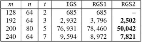
Table 1 Runtime for solving ideal lattice SVP (in seconds). The result of this paper is represented by bold font.

m n t GS IGS RGS1^† RGS2^†

128 64 2 7,432 18 17 –

192 64 3 3,423 129 113 73

200 80 5 904,860 98,581^∗ 89,502^∗ 52,164^∗

240 64 7 5,127 745^∗ 666^∗ 455^∗

∗usingt-nomial lattice

†using ImprovedReduceRot function

which the norm decreased over 10⁵ executions. Figure 7 shows thatp(t) approximated the experimental value almost correctly. We also confirmed that the probability of a de- crease in the norm decreases astincreases. Thus, the larger the value oftis, the more easily the norm tends to increase per a rotation, and the optimal number of rotationstis con- sidered to be small.

We generalize the discussion above from one rota- tion tok-fold rotations. Assume that the norm of the vec- tor v increases to ckvk or decreases to kvk/c per a ro- tation (c > 1). When we rotate a vector v k times, an important factor of success of a reduction is that the normkrot^k(v)kdoes not increase significantly from v and it stays in a certain range. Let Pk(t) be the probabil- ity that krot^k(v)k satisfies kvk/c ≤ krot^k(v)k ≤ ckvk for k. By using p(t) in Theorem 3, Pk(t) is written as P_k(t)=_k

d^k₂e p(t)^dk2e(1−p(t))^b2kc+p(t)^bk2c(1−p(t))^dk2e . For a threshold τ, we compute the maximum k that satisfies P_k(t) ≥ τ. Whenτ = 0.3,kis theoretically derived that is closer to the experimental value ofkas follows, whent=3 thenk=15, whent=5 thenk=5, when 7≤t ≤17 then k=3, when 18≤t≤33 thenk=2, and when 34≤tthen k=1. At least one rotation is valid for speeding up the GS for any dimension.

We compared the average runtime between the pro- posed algorithm and the existing algorithms for 10 execu- tions. The results are displayed in Table 1. We imple- mented theGS, the IGS with the ReduceInverseRot function (IGS), the RGS without the inverse rotation for the reduction (RGS1), and the RGS with the inverse rotation (RGS2). The cyclotomic polynomials for eachmare,Φ128(x)= x⁶⁴+1, Φ192(x)=x⁶⁴−x³²+1,Φ200(x)=x⁸⁰−x⁶⁰+x⁴⁰−x²⁰+1 andΦ240(x) = x⁶⁴ +x⁵⁶ −x⁴⁰ −x³² −x²⁴ +x⁸ +1. For t > 3, we implementedt-nomial rotation/inverse rotation inIGSand compared the runtime with those of RGS1 and RGS2under the same conditions. We used the optimal num- ber of rotationskobtained in the previous experiment. For t=2, since the inverse rotation is useless because we rotate a vector until reaching its period,IGSuses the ReduceRot function instead, and we omitRGS2. Table 1 shows that RGS1 is faster thanGSandIGSneverthelessRGS1 did not use the inverse rotation. The main reason is that the pro- cess of copying vectorvinIGSrequired much more time in practice than the rotation without it in RGS1. More- over,RGS2is approximately 1.5 times faster thanRGS1, as the ImprovedReduceRot function enables a reduction in the vectoruby inverse rotations without additional cost to pre-

Table 2 List size|L|(# of sampled vectors) ofIGS,RGS1andRGS2. The boldfont represents the smallest one.

m n t IGS RGS1 RGS2

128 64 2 685 685 –

192 64 3 2,932 3,796 2,502 200 80 5 76,931 78,460 50,042 240 64 7 9,594 8,972 7,821

pare an extra vectorv⁰⁰for the inverse rotation. The function leverages the inverse rotation for the reduction more effi- ciently than does the ReduceInverseRot function. Table 1 also implies that the t-nomial lattice is useful for not only our algorithm, but also others such asIGSbased on the GS.

For the same dimension, the smallertis, the smaller the run- time due to the cost of the rotation fortand the probability of decreasing the norm by a rotation. We presented the first time that GS could be sped up fort>3.

The space complexity is bounded by the list size ofL, in which Gauss-reduced and relatively shorter lattice vectors are contained. We measured the average list size of IGS, RGS1 andRGS2for 10 executions. The results are showen in Table 2. Whent = 2, no difference exists betweenIGS andRGS. For other values oft,RGS2is the smallest among the algorithms. However,RGS1 is not always smaller than IGS. The main reason is that the probability of a collision is higher when one uses the inverse rotation for the reduction.

6. Conclusion

In this paper, we defined t-nomial lattices as a generalized expression of anti-cyclic lattices, prime cyclotomic lattices, and trinomial lattices. Then, we designed the rotation oper- ation and the inverse rotation operation fort-nomial lattices by unraveling the relationship between the dimensionn of the input vectors,Φm(x) andt, i.e., the number of terms of Φm(x). We applied the rotation and inverse rotation struc- tures oft-nomial lattices to the IGS, and showed that it could reduce the computational time of the GS regardless of the dimensions. Moreover, we proposed RGS algorithm that could reduce the overhead caused by the copying of vectors in the IGS. Our experimental results suggested that the RGS was more than 1.5 times faster than the IGS.

References

[1] M. Ajtai, “The shortest vector problem inL₂isNP-hard for random- ized reductions,” Proc. thirtieth annual ACM symposium on Theory of computing, pp.10–19, 1998.

[2] M. Pohst, “On the computation of lattice vectors of minimal length, successive minima and reduced bases with applications,” SIGSAM Bull., vol.15, no.1, pp.37–44, 1981.

[3] M. Ajtai, R. Kumar, and D. Sivakumar, “A sieve algorithm for the shortest lattice vector problem,” Proc. Thirty-third Annual ACM Symposium on Theory of Computing, STOC’01, pp.601–610, ACM, 2001.

[4] D. Micciancio and P. Voulgaris, “Faster exponential time algorithms for the shortest vector problem,” Proc. Twenty-first Annual ACM- SIAM Symposium on Discrete Algorithms, SODA’10, pp.1468–

1480, SIAM, 2010.

[5] L. Ducas, “Shortest vector from lattice sieving: A few dimensions

for free,” Advances in Cryptology – EUROCRYPT 2018, pp.125–

145, Springer, 2018.

[6] M.R. Albrecht, L. Ducas, G. Herold, E. Kirshanova, E.W. Postleth- waite, and M. Stevens, “The general sieve kernel and new records in lattice reduction,” Advances in Cryptology – EUROCRYPT 2019, pp.717–746, Springer, 2019.

[7] S. Garg, C. Gentry, and S. Halevi, “Candidate multilinear maps from ideal lattices,” Advances in Cryptology – EUROCRYPT 2013, pp.1–

17, Springer, 2013.

[8] J. Hoffstein, J. Pipher, and J. Silverman, “NTRU: A ring-based pub- lic key cryptosystem,” Algorithmic Number Theory, pp.267–288, Springer, 1998.

[9] M. Schneider, “Sieving for shortest vectors in ideal lattices,”

Progress in Cryptology – AFRICACRYPT 2013, pp.375–391, Springer, 2013.

[10] T. Plantard, W. Susilo, and Z. Zhang, “LLL for ideal lattices: re- evaluation of the security of Gentry–Halevi’s FHE scheme,” Des.

Codes Cryptogr., vol.76, pp.325–344, 2015.

[11] A.K. Lenstra, H.W. Lenstra, and L. Lov´asz, “Factoring polynomials with rational coefficients,” Math. Ann., vol.261, no.4, pp.515–534, 1982.

[12] T. Ishiguro, S. Kiyomoto, Y. Miyake, and T. Takagi, “Parallel Gauss sieve algorithm: Solving the SVP challenge over a 128-dimensional ideal lattice,” Public-Key Cryptography – PKC 2014, pp.411–428, Springer, 2014.

[13] V. Lyubashevsky, C. Peikert, and O. Regev, “On ideal lattices and learning with errors over rings,” Advances in Cryptology – EURO- CRYPT 2010, pp.1–23, Springer, 2010.

[14] H. Riesel, Prime Numbers and Computer Methods for Factorization, pp.305–308, Birch¨auser, 1994.

[15] P. Klein, “Finding the closest lattice vector when it’s unusually close,” Proc. Eleventh Annual ACM-SIAM Symposium on Discrete Algorithms, SODA’00, pp.937–941, SIAM, 2000.

[16] T. Nagell, Introduction to Number Theory, pp.158–168, Wiley, 1951.

[17] L. Carlitz, “The number of terms in the cyclotomic polyno- mial Fpq(x),” The American Mathematical Monthly, vol.73, no.9, pp.979–981, 1966.

[18] A. Migotti, “Zur Theorie der Kreisteilungs-gleichung,” S.-B. der Math.-Naturwiss. Class der Kaiser. Akad. Der Wiss., Wien, vol.87, pp.7–14, 1883.

[19] P. Voulgaris, “A simple implementation in C++of Gauss Sieve,”

https://cseweb.ucsd.edu/˜pvoulgar/impl.html

Shintaro Narisada received his B.E. in Electrical, Information and Physics Engineering and his M.E. in Information Sciences from To- hoku University, Japan, in 2016 and 2018, re- spectively. He joined KDDI in 2018 and has been engaged in the research on lattice-based cryptography. He is currently an associate re- search engineer at the Information Security Lab- oratory of KDDI Research, Inc.

Hiroki Okada received his B.E. and M.E.

in applied mathematics and physics from Kyoto University, Japan, in 2014 and 2016, respec- tively. He joined KDDI in 2016 and has been en- gaged in research on lattice-based cryptography and homomorphic encryption. He is currently an associate research engineer at the Informa- tion Security Laboratory of KDDI Research, Inc.

Kazuhide Fukushima received his M.E.

in Information Engineering from Kyushu Uni- versity, Japan, in 2004. He joined KDDI and has been engaged in the research on post- quantum cryptography, cryptographic protocols, and identification technologies. He is currently a research manager at the Information Security Laboratory of KDDI Research, Inc. He received his Doctorate in Engineering from Kyushu Uni- versity in 2009. He received the IEICE Young Engineer Award in 2012. He served as the Ed- itor of IEICE Transactions on Fundamentals of Electronics Communica- tions and Computer Sciences from 2015 to 2017, and he is a Director, General Affairs of IEICE Engineering Science Society from 2019. He is a member of the Information Processing Society of Japan.

Shinsaku Kiyomoto received his B.E.

in engineering sciences and his M.E. in Ma- terial Science from Tsukuba University, Japan, in 1998 and 2000, respectively. He joined KDD (now KDDI) and has been engaged in research on stream ciphers, cryptographic pro- tocols, and mobile security. He is currently a senior researcher at the Information Security Laboratory of KDDI Research, Inc. He was a visiting researcher of the Information Security Group, Royal Holloway University of London from 2008 to 2009. He received his doctorate in engineering from Kyushu University in 2006. He received the IEICE Young Engineer Award in 2004 and Distinguished Contributions Awards in 2011. He is a member of IEICE and JPS.