Evaluation of Non‑Survey International IO Construction Methods with the Asian‑Pacific Input‑Output Table
著者 Oosterhaven Jan, Stelder Dirk, Inomata Satoshi
権利 Copyrights 日本貿易振興機構(ジェトロ)アジア
経済研究所 / Institute of Developing
Economies, Japan External Trade Organization (IDE‑JETRO) http://www.ide.go.jp
journal or
publication title
IDE Discussion Paper
volume 114
year 2007‑07‑01
URL http://hdl.handle.net/2344/641
INSTITUTE OF DEVELOPING ECONOMIES
IDE Discussion Papers are preliminary materials circulated to stimulate discussions and critical comments
Keywords: Non-survey estimates, international trade, input-output tables, East-Asia JEL classification: C81, D57, R15
* Oosterhaven and Stelder are, respectively, professor and assistant professor of spatial economics at the RUG. Inomata is the director of the Asian International Input-Output Project of IDE/JETRO. Corresponding address: [email protected]
IDE DISCUSSION PAPER No. 114
Evaluation of Non-Survey International IO Construction Methods with the
Asian-Pacific Input-Output Table
Jan Oosterhaven, Dirk Stelder and Satoshi Inomata *
July 2007
Abstract
This paper presents four non-survey methods to construct a full-information international input-output table from national IO tables and international import and export statistics, and this paper tests these four methods against the semi-survey international IO table for nine East-Asian countries and the USA, which is constructed by the Institute of Developing Economies in Japan.
The tests show that the impact on the domestic flows of using self-sufficiency ratios is small, except for Singapore and Malaysia, two countries with large volumes of smuggling and transit trade. As regards the accuracy of the international flows, all methods show considerable errors, of 10%-40% for commodities and of 10%-70% for services. When more information is added, i.e. going from Method 1 to 4, the accuracy increases, except for Method 2 that generally produces larger errors than Method 1. In all, it seems doubtful whether replacing the semi-survey Asian-Pacific IO table with one of the four non-survey tables is justified, except when the semi-survey table itself is also considered to be just another estimate.
The Institute of Developing Economies (IDE) is a semigovernmental, nonpartisan, nonprofit research institute, founded in 1958. The Institute merged with the Japan External Trade Organization (JETRO) on July 1, 1998.
The Institute conducts basic and comprehensive studies on economic and related affairs in all developing countries and regions, including Asia, the Middle East, Africa, Latin America, Oceania, and Eastern Europe.
The views expressed in this publication are those of the author(s). Publication does not imply endorsement by the Institute of Developing Economies of any of the views expressed within.
INSTITUTE OF DEVELOPING ECONOMIES (IDE), JETRO 3-2-2, WAKABA,MIHAMA-KU,CHIBA-SHI
CHIBA 261-8545, JAPAN
©2007 by Institute of Developing Economies, JETRO
Evaluation of Non-Survey International IO Construction Methods with the Asian-Pacific Input-Output Table
Jan Oosterhaven, Dirk Stelder and Satoshi Inomata 1
Paper for the 16th International Input-Output Conference, Istanbul, July 2007
Abstract
This paper presents four non-survey methods to construct a full-information international input-output table from national IO tables and international import and export statistics, and this paper tests these four methods against the semi-survey international IO table for nine East-Asian countries and the USA, which is constructed by the Institute of Developing Economies in Japan.
The first method assumes that the national IO tables do not contain a distinction between domestic and imported intermediate inputs and final demand. The split-up of the national table into these two subtables is made by using aggregate self-sufficiency ratios by sector by country. The three other methods assume that this split-up is already made in the national IO tables. All four methods proceed by the further split-up of the IO import tables over the countries of origin using import ratios derived from the imports trade statistics. In the first two methods, the necessary re-pricing of the imports from ex customs’ prices into producers’ prices and the balancing of the split-up import tables with the aggregate IO export columns is done by applying the GRAS algorithm.
In the third method, this re-pricing and balancing is done at the level of the block column matrix with imports per purchasing country. The row totals are derived by applying the export trade destination ratios to the aggregate IO export columns. The fourth method also uses these estimated bilateral export columns, but replaces their implicit country origins with the country origins of the import submatrices.
The tests show that the impact on the domestic flows of using self-sufficiency ratios is small, except for Singapore and Malaysia, two countries with large volumes of smuggling and transit trade. As regards the accuracy of the international flows, all methods show considerable errors, of 10%-40% for commodities and of 10%-70% for services. When more information is added, i.e. going from Method 1 to 4, the accuracy increases, except for Method 2 that generally produces larger errors than Method 1. In all, it seems doubtful whether replacing the semi-survey Asian-Pacific IO table with one of the four non-survey tables is justified, except when the semi-survey table itself is also considered to be just another estimate.
Keywords
Non-survey estimates, international trade, input-output tables, East-Asia, Pacific
1 This paper presents the results of a research project commissioned by the Institute of Developing Economies (IDE/JETRO) in Japan to the University of Groningen (RUG) in the Netherlands. Oosterhaven and Stelder are, respectively, professor and assistant professor of spatial economics at the RUG. Inomata is the director of the Asian International Input-Output Project of IDE/JETRO. Corresponding address: Faculty of Economics, University of Groningen, Postbus 800, 9700 AV Groningen, the Netherlands, fax +31-50-363.7337, email [email protected].
1. Introduction
International input-output data are indispensable for solid research into such phenomena as the international fragmentation of production processes, the relative importance of intra-industry trade versus interindustry trade, international comparisons of total factor productivity, and the construction of international input-output (IO) and computable general equilibrium models. The construction of internally consistent, survey-based international IO tables, however, is extremely expensive. It is, therefore, paramount to systematically investigate whether the non-survey construction of such tables would not present a viable alternative. There is, however, little information on and experience with non-survey international IO construction methods that we know of.
In this paper, we aim at providing such information, using the semi-survey international Asian-Pacific IO table for 2000 (IDE, 2006) as a benchmark, while extending earlier comparable work for the European Union (van der Linden & Oosterhaven, 1995).
As opposed to non-survey international IO construction methods, there is a whole literature on non-survey single region methods (see Batten & Martellato, 1985, and Canning & Wang, 2005). In this literature, Boomsma & Oosterhaven (1992) plea to use the double-entry properties of a bi-regional IO accounting framework to avoid the systematic tendency to overestimate the intra-regional transactions that is present in most non-survey single region methods. Oosterhaven (2005a), additionally, shows how an interregional setup is useful when spatially disaggregating national IO tables or multipliers.
In the case of international IO tables, the problem of overestimating domestic transactions is hardly present, as the main problem then is the integration of survey- based national tables by means of survey-based trade statistics, which type of data is usually absent when constructing interregional tables. In the international case, using the double-entry character of IO accounting implies using import as well as export data from both IO tables and trade statistics, while solving the various discrepancies between them. The most important and most systematic of these discrepancies is the difference between the valuation of IO exports in producers’ prices and the valuation of IO imports in ex customs’ prices.
Van der Linden & Oosterhaven (1995), in essence, offer a two-step solution for this problem in the case of the European Union Intercountry IO tables. Their first step essentially disaggregates each country’s IO import table by origin, using bilateral import trade statistics, while their second step essentially re-prices these imports from ex customs’ prices to producers’ prices, using RAS. Their solution, however, ignores data from export trade statistics. In this paper, we will take their approach one important step further by also using bilateral export trade statistics. In addition, we will also consider the frequently occurring case of national IO tables that do not separate foreign imports from domestic use and investigate the errors made when this information is absent.
To test the various non-survey methods, we will use the unique set of detailed national IO tables with 76 sectors and 4 final demand categories, with and without the separation of foreign imports from domestic use, together with the import and export trade statistics of nine Asian countries and the USA for 2000, as harmonized by the Institute of Developing Economies in Japan (IDE, 2006, see especially Inomata et al.
2006). With these data we will construct four successively less non-survey Asian- Pacific International IO Tables (AIOTs) and compare them, using several distance measures, with the semi-survey AIOT constructed by IDE (2006, see also Meng et al.
2006).
Section 2 will explain the accounting setup of the ideal international IO table and summarize the non-survey method developed for the European Union by van der
Linden & Oosterhaven (1995). Section 3 explains how and where the AIOT construction method differs from the EU method, and why the AIOT has to be labeled as a semi-survey table. Section 4 will explain how the EU-method will be adapted to the Asian-Pacific data from IDE (2006), which gives our second non-survey method.
Taking the EU-method one step back and two steps forward produces our first, third and fourth non-survey method. Section 5 will compare the four successively less non- survey AIOTs with the IDE semi-survey AIOT at the level of its intercountry cells, at the level of its intercountry row and column totals, and at the level of the intercountry spillovers that may be derived from the intercountry IO model (Oosterhaven, 1981).
Section 6 concludes.
2. The EU non-survey intercountry IO construction method
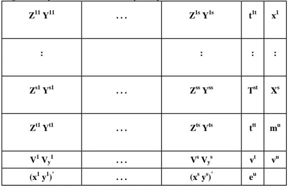
The most complete international input-output table2 contains full information on the sectoral and national origin as well as on the sectoral and national destination of each intermediate demand flow z and each final demand flow y. Figure 1 shows the layout of such an ‘ideal’ international table for s countries, which in this case together form the European Union.3
Besides the transactions within the Union there are of course transactions with third countries t outside the Union. Figure 1 shows the imports from third countries in the form of full intermediate input Zts matrices and full final demand Yts matrices per sector of origin within the rest of the world (ROW), where s indicates the country of destination. This detail on the sectoral origin is necessary if one wants to calculate the real technical coefficients of sector j in country s, as these have to show the need for the worldwide inputs of a specific commodity i per unit of output of sector j in country s:
/x z / x z ) z + ( x = / z ) z + z + (
a = sj
s ij s
j us ij ts ij s
j ss ij os ij ts ij s ij
= • (1)
where i and j indicate the sectors of origin and destination, ts = imports from third countries outside the Union into country s, os = imports from the other countries within the Union into s, ss = domestic inputs, us = total inputs from within the Union, and •s = total inputs from all over the world.
The •s-data are the point of departure of our first non-survey method, and the us- data are the point of departure of the three other non-survey methods.
In the case of exports to third countries comparable detail about the sectoral destination is analytically not necessary, which implies that one export column per country or origin r (trt) is sufficient. The same holds for the transit of products from third countries through the Union to other third countries (ttt).
Note that the well-known macro-economic accounting identity not only holds for the national IO table of each country s (Ys = Cs + Is + Gs + Es – Ms), but also for the IO table of the Union as a whole. In the latter case, however, Union exports and Union imports have to be defined with regard to third countries outside the Union (cf. Figure 1):
Yu = ∑s Vs + ∑s Vys + vt = vu = ∑s ys + eu – mu = Cu + Iu + Gu + Eu – Mu (2)
2 See Isard (1951) for the ‘ideal’ table and Oosterhaven (1984) for a description of the full family of interregional IO tables.
3 For the European Union, various intercountry tables have been constructed for different years with different numbers of member countries.
where ys = Cs + Is + Gs, the total of the domestic part of the final demand of each country s.
Figure 1. Layout of the international input-output table with full information.
Z11 Y11 . . . Z1s Y1s t1t x1
: : : :
Zs1 Ys1 . . . Zss Yss Tst Xs
Zt1 Yt1 . . . Zts Yts ttt mu
V1 Vy1 . . . Vs Vys vt vu
(x1 y1)’ . . . (xs ys)’ eu
Constructing a full information international IO table from regular national IO tables and international trade statistics is problematic as the import data and the export data in these two sources do not match. There is a series of registration discrepancies (see van der Linden, 1998, for an extensive discussion). The most important discrepancy has a systematic source as different prices are used to value the imports and exports in the two data sources. Figure 2 shows these systematic differences and also shows that the difference between the IO imports and the IO exports must be largest (as is confirmed by table 1 in Van der Linden & Oosterhaven, 1995). Solving that valuation discrepancy is therefore the most important task of any non-survey international IO table construction procedure.
Figure 2. Price definitions used in valuating international trade flows.
Basic price (production cost) in country r + Indirect taxes in country r =
Producers’ price in country r
+ Trade and transport margins in country r =
→ Export value in IO tables Free on Board (f.o.b.) price leaving country r
+ trade and transport margins between r and s =
→ Export value in trade statistics Cost, Insurance and Freight (c.i.f.) price for country s
+ Indirect taxes in country s =
→ Import value in trade statistics
Ex customs’ price for country s → Import value in IO tables
In the case of the European Union, five non-survey intercountry IO tables for 1965- 1985 (van der Linden & Oosterhaven, 1995) were constructed combining Eurostat’s harmonized national IO tables that consist of four subtables (see e.g. Eurostat, 1983, 1986) with Eurostat’s import trade statistics (see Eurostat, 1990). The EU-construction method essentially proceeds along the following steps (see van der Linden, 1998, for full details):
1. The IO subtables with primary inputs Vs and Vys, total output xs and total final demand ys are directly put into the corresponding submatrices and subvectors of
Figure 1.
2. The IO subtables with domestic transactions measured in producers’ prices are directly put into the diagonal submatrices Zrr and Yrr of Figure 1.
3. The IO subtables with imports from non-EU countries measured in ex customs’
prices are directly put into the third country import submatrices Ztr and Ytr of Figure 1.
4. The IO subtables with imports from EU-countries measured in ex customs’ prices Zos and Yos are disaggregated row-wise by EU-country of origin by means of import ratios calculated from the Eurostat import statistics, and are then put into an auxiliary EU-internal trade matrix M.
5. The internal and external EU-transit trade columns from the subtables mentioned under 2-4 are distributed over the appropriate subtables or are directly put into ttt in Figure 1.
6. The columns with the exports to ROW-countries measured in producers’ prices are directly put into the trt columns in Figure 1.
7. The columns with the exports to other EU-countries measured in producers’ prices tro are re-scaled to match the overall total of the auxiliary EU-internal trade matrix M. The difference of about 1% is added as a re-scaling column to Figure 1.
8. The auxiliary matrix M measured in ex customs’ prices is iteratively re-scaled by means of RAS such that its row totals match the re-scaled columns with the exports to EU-countries measured in producers’ prices, and the result is put in the corresponding submatrices Zrs and Yrs of Figure 1.
The two crucial steps are step 4 and step 8. Step 4 adds the lacking spatial origin to the Eurostat intra-EU import matrices and step 8 re-prices the Eurostat intra-EU import matrices from ex customs’ prices to producers’ prices.
This last step is needed for two reasons. First, it is needed to produce an internally price-consistent consolidated EU-table to replace the present inconsistent, consolidated EU-tables (e.g. Eurostat, 1983, 1986). Second, it is needed to correctly allocate the impacts of any change in final demand to the foreign sectors that really produce the imported intermediate inputs. In absence of step 8, intercountry spillovers and feedbacks on the trade and transport sectors would be grossly under-estimated, whereas intercountry impacts on especially the primary and secondary sectors would be systematically over-estimated.
3. The Asian-Pacific intercountry IO construction method
The AIOT should be categorised as a “semi-survey table”. It is certainly not a non-survey table because it embodies two extensive surveys conducted by the collaborating institutions of the AIOT project, yet it is neither a full-survey table because the separation of import matrix by country of origin, which forms a major aspect of constructing intercountry tables, is mechanically done by using the country shares of import statistics, instead of conducting and utilising the survey on domestic distribution of imported goods and services by country of origin.
The construction of the AIOT is a time and resource consuming process, and four to five years are usually spent in order to complete the table. The construction steps, however, resembles the method using in the estimation of the EU intercountry tables. To avoid the repetition with the previous section, it is extended here only to point out some of the major differences with the EU counterpart.4
4 For more detailed description of the AIOT construction method, see Inomata et al. (2006).
3.1 Harmonization of the constituent national tables
Despite the fact that input-output tables constitute the central apparatus of the System of National Accounts, each national table of the AIOT countries exhibits more or less different features and characteristics, reflecting each country’s economic idiosyncrasies and availability of data. Accordingly, the presentation style of national tables must be manually adjusted towards the common AIOT format. In general, it are the detailed, information-rich tables that have to concede to the less-detailed ones, as the other way round would require a costly effort of obtaining supplementary data. So, there always exists a trade-off between the level of uniformity and the level of information, and hence a careful and thorough consideration is called for in making adjustment rules. Figure 3 shows a list of adjustment targets for each AIOT national tables. This is indeed the most complicated, nerve-racking phase of the construction, yet without this harmonization process the constituent tables cannot form the AIOT such that the interpretation of the data is mutually consistent and comparable for any part of the whole.
Figure 3. List of adjustment targets for each national input-output table*
IND MYS PHL SNG THA CHN TWN KOR JPN USA
1. Conversion of valuation
1.1 Basic price to producer's price X
1.2 Private consumption expenditure X X X
1.3 Export vectors X X
1.4 Import matrix/vector X X X X X
2. Negative entries X
3. Dummy sectors X X X X X X
4. Machine-repair X X X X
5. Financial intermediaries X X X X
6. Special treatment of import/export
6.1 Water transportation X
6.2 "Pure import" of gold X
6.3 Re-export X
6.4 Telecommunication X
7. Computer software products X
8. Producers of government services X X
* From left to right in the list: Indonesia, Malaysia, Philippines, Singapore, Thailand, China (mainland), Taiwan, Korea, Japan, the USA.
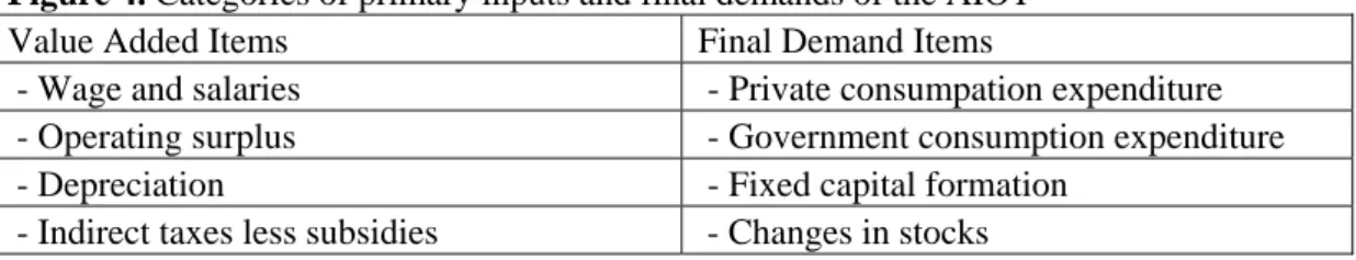
Figure 4. Categories of primary inputs and final demands of the AIOT
Value Added Items Final Demand Items
- Wage and salaries - Private consumpation expenditure - Operating surplus - Government consumption expenditure - Depreciation - Fixed capital formation
- Indirect taxes less subsidies - Changes in stocks
3.2 Derivation of import matrices and export columns by origin/destination The information on the use of imported goods and services is crucial for constructing intercountry tables. In order to present import transactions separately from the transactions of domestic products, statistical offices of the AIOT countries
conduct an extensive survey on the domestic distribution of imported inputs. On this account, each row in the import matrix thus produced can individually tell us which domestic industry uses that particular imported item by what amount, the structure of which is apparently considered different from that of the domestic transaction sub- table. This is the first point where the survey comes in over the AIOT construction process, given that the national I-O table without import matrix (dubbed as
“competitive-import type” table) is our start line.
The valuation of the import matrix differs between the tables. Some country’s tables contain import duties and import commodity taxes in each transaction value, while others do not. So, for the former case, the taxes on import have to be separated out using the rates of import duties and import commodity taxes. The separated matrix of duties and taxes is then aggregated column-wise to form a single row vector, which is to be placed below the import matrix from the rest of the world.
The c.i.f. import matrices thus derived, however, do not differentiate the imported inputs from the Asia-Pacific region and those from the rest of the world, as the EU counterparts do. So, although the construction of the AIOT follows Steps 1 and 2, as presented in the previous section, the Step 3 becomes the point of departure from the EU method. While the EU method simply transplants the given import sub- tables from non-EU countries into import sub-matrices Ztr and Ytr, the AIOT obtains the import matrix from the rest of the world as a “residual” of ripping off all the import matrices from the AIOT countries, following the disaggregation of the import matrix by country of origin (i.e. Step 4 in the EU method.) The dichotomy also applies to Step 6, the making of export vector to the rest of the world.
This brings us to a crucial difference between the AIOT and the EU table. Some countries of the AIOT members, i.e. Korea, Taiwan, the Philippines, Singapore and Thailand, do not have any external source of data on service trade with origin / destination information. In that case, the disaggregation of the import matrix by origin (and the export vector by destination) is done just by referring to the custom trade statistics which cover only goods transactions. As a result, the service trade is not disaggregated and hence all the service transaction values, except those of the trade and transport sectors, are to be recorded in the import matrix from (and the export vector to) the rest of the world.
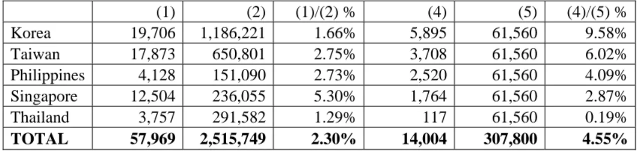
This has an important implication for the comparison exercises in section 5 of the paper; that is, the IDE’s semi-survey table will systematically underestimate the non-survey table based on the EU method for the service sectors of some inter- country transaction matrices. However, as shown in Figure 5, such a systematic underestimation will occur in the cells which constitute only 4.55 % of the entire matrix, and in terms of values, only 2.30% of all transactions, reflecting the negligible scale of service trade for the countries concerned.
Figure 5. Value and number of entries in service transactions systematically underestimated
(1) (2) (1)/(2) % (4) (5) (4)/(5) %
Korea 19,706 1,186,221 1.66% 5,895 61,560 9.58%
Taiwan 17,873 650,801 2.75% 3,708 61,560 6.02%
Philippines 4,128 151,090 2.73% 2,520 61,560 4.09%
Singapore 12,504 236,055 5.30% 1,764 61,560 2.87%
Thailand 3,757 291,582 1.29% 117 61,560 0.19%
TOTAL 57,969 2,515,749 2.30% 14,004 307,800 4.55%
(1) Underestimated value of service import in AIOT (million US$) (2) Total value of domestic and import transactions in AIOT (million US$) (4) Number of entries in service import systematically underestimated (5) Total number of cells in the whole matrix: 760 rows x 81 columns
3.3 Re-pricing of import matrices and final reconciliation
From the step 7 onwards, the EU method proceeds to re-pricing import matrices from ex custom’s price to producer’s price, using re-scaled export data and RAS algorithm. The AIOT, on the other hand, conducts an extensive study to bridge between the two pricing schemes, though the AIOT’s import matrices at this stage are already free of import duties and import commodity taxes, and hence valued at c.i.f.
instead of ex custom’s price. What we need, therefore, are the data of trade and transport margins for the delivery of exported goods (from factories to ports), and the data of international freight and insurance costs levied on the shipping of items between the countries, as indicated by Figure 2.
Usually the data of trade and transport margins on exports can be obtained from the supporting matrix of national IO tables. If not, a special survey might be called for.
Yet in the case that the survey is unfeasible or inappropriate, the average figures of the delivery margins between domestic industries are used as proxies.
As for international freight and insurance costs, the raw data are directly collected from the custom trade statistics wherever possible. The data are obtainable for all the AIOT countries except Taiwan, but their quality varies across the countries and some individual transaction values are often missing in the tabulation.
Here again, it is required to conduct a spot survey and to apply some estimation methods to make up for the missing information, which is done in two steps. Firstly a regression model is run for each of the traded goods, by taking the shipping distance between countries as a proxy for shipping costs. After obtaining the parameter estimates for the equation, the missing values are projected upon the estimated model.
With this specially collected and estimated information, the AIOT’s import matrices are converted into producer’s price, which completes the construction process after due balancing exercises.
4. The four non-survey AIOT methods
First, we present a base variant of the EU-method that may be applied to the harmonized national AIOT tables without an import matrix, which are labeled as
‘competitive import type’ tables by IDE (2006). Second, we show how the original EU- method has to be adapted to be applied to national AIOT tables with a separate import matrix, which are labeled as ‘non-competitive import type’ tables by IDE (2006). Third, we develop a new method that not only uses information from the import trade statistics but also from the export trade statistics. Fourth, we develop a new method that uses the sectoral origin information from the export trade statistics, but replaces their spatial destination information with that derived from the import trade statistics. Finally, we compare the rescaling factors that are used to make the export data consistent with the import data before the GRAS balancing algorithm (Junius & Oosterhaven, 2003) is applied.
All four methods start with filling up the bottom rows of figure 1 with the AIOT primary input data and the last column of figure 1 with the AIOT exports to non-AIOT countries, i.e. with step 1 of the EU-method.
4.1 Non-survey method for national IO tables without import matrices
Our first non-survey method then proceeds with allocating the import duties’
columns of the ten national IO tables without import tables from IDE (2006) ( ) to the purchasing sectors and final demand categories q in each country s, after which they are
s
di
aggregated into ten single sub-rows:
s d q
z z
d = i si
s i s iq s
q
∑
( • / •• ) ∀ , (3)where i and q run from 1 to 76 for intermediate demand and q runs further from 77 to 80 for domestic final demand.5 A ‘•’ indicates a summation over the index concerned.
The results of (3) are put in the appropriate primary input sub-rows of Figure 1, which finishes step 1.
Second and most importantly, we estimate the domestic intermediate and final transactions, and , as if they were not known. This is done by using the aggregate self-sufficiency ratios from the ten national IO tables without import tables:
ss
zij yifss
s q z i
z m z
z = iqs
s i s i s i ss
iq [( •• − )/ •• ] • ∀ , , (4)
where indicates the import of products i according to the IO table of country s. Note that (4) implicitly assumes that transit flows through country s are zero. The results of (4) are put in the ten appropriate diagonal sub-matrices of Figure 1, analogous to step 2 of the EU-method.
s
mi
Next, the ten implicitly estimated import matrices result by taking the difference between the ten ‘competitive import type’ national IO tables from IDE (2006) and the above estimated ten diagonal submatrices:
s q z i
=z m
m iqss
s iq ts iq os
iq + • − ∀ , , (5)
The remainder of our first non-survey method, from hereon, exactly follows the same steps as our second non-survey method.
4.2 The EU-method adapted to the Asian-Pacific tables with import matrices Our second non-survey method starts with taking the data defined in (4) and (5) directly from the ten ‘competitive import type’ tables from IDE (2006).
The EU-steps 3 and 4 have to be adapted a little as the split-up of the import matrices (5) between the other nine Asian-Pacific countries and the ROW is not known in the case of the ten AIOT-countries. For the first 61 commodity sectors, this split-up is made by using the import origin ratios ) for products i per importing country s from the import trade statistics from IDE (2006):
/ (m mis
rs i
••
•
q i
s s m r
m m m
m tsiq
os iq s i rs i rs
iq =( •/ ••)( + ) ∀ ≠ , , ≤61, (6)
where r and s run from 1 to 10 and r runs further from 11 to 13.6
For the remaining 15 service sectors, no trade statistics are available. The lacking services import ratios are therefore assumed to be equal to the total of the commodity sectors:
5 With 77 = private consumption, 78 = government consumption, 79 = gross domestic fixed captial formation, 80 = change in stocks.
6 With 1 = Indonesia, 2 = Malaysia, 3 = Philippines, 4 = Singapore, 5 = Thailand, 6 = China, 7
= Taiwan, 8 = South Korea, 9 = Japan, 10 = USA, 11 = Hong Kong, 12 = EU-15, 13 = ROW.
q i
s s m r
m m m
m tsiq
os iq s rs rs
iq =( ••/ •••)( + ) ∀ ≠ , , ≥62, (7)
This assumption is especially reasonable for the imports of trade and transport services, as these are defined as the margins on the commodities that are actually imported (see Figure 2).
For each of the ten AIOT-countries, the three import submatrices for r = 11-13 are aggregated column-wise into three rows, which are then put in the appropriate third country imports submatrices of Figure 1, analogous to EU-step 3. The nine remaining import submatrices are put into the auxiliary intercountry imports matrix M, analogous to EU-step 4. As the Asian-Pacific national IO tables from IDE (2006) do not contain columns of row with transit trade, EU-step 5 is not needed in case of the non-survey construction of the AIOT.
EU-steps 6 and 7 also have to be adapted a little as the split-up of the ten national export columns into a column for the other nine Asian-Pacific countries and a column for the ROW is not given in the national IO tables from IDE (2006). For the first 61 commodity sectors, this split-up is made by using the export destination ratios
per exporting sector i per country r from the export statistics from IDE (2006):
) / (e eir
rs i
•
61 ,
, )
/
( ∀ ≠ ≤
= e e• t r s r i
t ri
r i rs i rs
i (8)
where r and s run from 1 to 10 and s runs further from 11 to 13.
For the lacking export destination ratios of the 15 service sectors again the total of the commodity sectors is taken:
62 ,
, )
/
( ∀ ≠ ≥
= e• e•• t r s r i
t ri
r rs rs
i (9)
This is again a reasonable assumption, especially for the exports of trade and transport services.
For each of the ten AIOT-countries, the three export columns for s = 11-13 are put in the exports sub-columns for exports to third countries in figure 1, analogous to EU- step 6.
From hereon our first two non-survey methods deviate from the last two methods.
Here, i.e. for our first and second method, we aggregate the export columns relating the nine other AIOT-countries into a single tro column for each of the AIOT-countries.
Next, these ten country columns are combined into one single extended column to. This column is then re-scaled to the overall total of the auxiliary intercountry imports matrix M, by means of , which equaled 1.27. This indicates that the total of the estimated IO imports between all AIOT-countries were 27% larger than the estimated total of the IO exports between these countries. The absence of transit trade and transit trade and transport margins in the original IDE (2006) tables may be part of the explanation of this large discrepancy, which in the case of the EU intercountry IO tables amounted to only about one percent of the intra-EU imports (van der Linden, 1998).
The 27% difference:
o
o t
m•••/ ••
i r t
t m
rir = (1− ••o• / ••o) iro ∀ , (10)
is put in a re-scaling column next to the three third country exports columns in Figure 1, analogous to EU-step 7.
The re-scaled to column subsequently serves as the row restriction for the RAS re- pricing of the auxiliary intercountry imports matrix M, as in EU-step 8. An important difference with the EU-method is that we do not use the original RAS procedure, but its generalization developed by Junius & Oosterhaven (2003, see also Oosterhaven, 2005b), as this generalization allows for negative cells and negative totals.7 By using GRAS the ten final demand columns with the partly negative changes in stocks (q = 80) do not have to be treated separately.
Note that using the re-scaled to as the row totals for the final intercountry import matrix M* implies not only a re-pricing of the original M, but also implies a rescaling of the import ratios of M such that they are consistent with the overall import ratios implicit in the original to aggregate exports column.
4.3 A non-survey method also using bilateral export data
The difference between the adapted EU-method and our first new method is the use of the individual columns with the estimated bilateral IO exports from (8)-(9). Instead of applying GRAS to the entire auxiliary intercountry import matrix M, we now apply GRAS to the block-column matrix with the nine import submatrices per purchasing country s, Ms = [M1s, … Ms-1,s, Ms+1,s, … M10,s]’. The column totals of the final Ms* will of course be equal to those of the original Ms, but its row totals will be made equal to the re-scaled column with the exports from the other nine AIOT-countries to AIOT- country s from (8)-(9):
ts = (m•os•/t•os)[t1s, … ts-1,s, ts+1,s, … t10,s]’ (11)
As a result we now have ten different re-scaling columns, with re-scaling factors varying per purchasing AIOT-country from 0.54 for Singapore to 1.48 for China (see Table 1); with their weighted average equaling the overall re-scaling factor of 1.27 needed with Method 2. The very low value for Singapore most likely indicates that AIOT-countries register a larger part of their transit exports through Singapore as exports with a final destination in Singapore, than they do register their transit imports from Singapore as imports being produced in Singapore. The large value for China, on the other hand, indicates that the imports from the AIOT-countries as estimated from the Chinese national IO table are much larger than the exports to China as estimated from the nine other national IO tables. The primary cause for this observation is the transit trade through Hong Kong, for which the AIOT-countries record the transactions as export to Hong Kong while China more correctly records them as import from AIOT countries based on the country of origin principle.
) / (m•os• t•os
Table 1. Re-scaling of the export columns per importing country in Method 3.
IND MYS PHL SNG THA CHN TWN KOR JPN USA MAD 1.24 1.20 0.77 0.54 1.12 1.48 1.10 1.15 1.23 1.15
In this case, the row-wise totals of these ten re-scaling columns:
∑
− ∀= •• •
s
rs i os os r
i m t t i r
r (1 / ) , (12)
are combined in a single column and are then put next to the three third country exports columns in Figure 1, analogous to EU-step 7.
7 The Junius & Oosterhaven (2003) method has been slightly revised, by removing e and e-1 for the algorithm, to cope with the problem noted in (Lenzen, Wood & Gallego, 2007).
Finally, the GRAS algorithm now has been run ten times for each of the purchasing countries s separately, instead of the single run of RAS in EU-step 8.
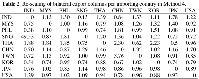
4.4 A non-survey method rescaling bilateral exports to bilateral imports
The question may be raised whether import trade statistics do not contain more reliable information on the spatial dimension of international trade than export trade statistics. If they do, it is better to replace the spatial dimension of the export statistics with that of the corresponding import statistics. Our fourth method precisely does that.
It re-prices the ten block-column matrices Ms = [M1s, … Ms-1,s, Ms+1,s, … M10,s] from the ex-customs’ prices of the IO import data to the producers’ prices of the IO export data, but it rescales the bilateral export columns to their corresponding value from the bilateral import sub-matrices of Ms, as follows:
ts = [(m1••s/t•1s)t1s, … (m•s•−1,s/t•s−1,s)ts-1,s, (m•s•+1,s/t•s+1,s)ts+1,s, … (m10••s/t10• s)t10,s]’ (13)
As a result we again get ten rescaling columns, but now each column s has nine different re-scaling sub-factors , which are shown in Table 2. The weighted average column totals of Table 2 of course equal the re-scaling factors from Table 1.
The largest re-scaling factor of 49.5 shows that the registration error for transit trade through Singapore most certainly originates from Indonesian imports being wrongly allocated to come from Singapore, as the alternative of Singapore exports not being allocated to Indonesia is much less likely. In this case, giving priority to the import data will deteriorate the quality of the Method 4 compared to Method 3. The smallest re- scaling factor of 0.13 for Indonesian exports to Singapore is equally interesting. It most likely originates from Indonesian exports being wrongly allocated to Singapore, whereas their final destination is further out. In this case, giving priority to the import data improves the quality of Method 4 above that of Method 3. The next largest ratio of 3.76 of Chinese imports from Taiwan, compared to Taiwanese exports to China, may also result from a transit trade registration error.
) / (m•rs• t•rs
This type of information could, in fact, be used to create a 5th method, but then the label non-survey would no longer be justified, as that method would require time consuming research into registration practices.
Table 2. Re-scaling of bilateral export columns per importing country in Method 4.
IND MYS PHL SNG THA CHN TWN KOR JPN USA
IND 0 1.13 1.30 0.13 1.39 0.84 1.33 1.11 1.78 1.22
MYS 0.75 0 1.00 1.16 0.79 1.08 1.26 1.32 1.40 0.92
PHL 0.38 1.10 0 0.99 0.74 1.81 0.99 1.51 1.08 0.91
SNG 49.53 0.87 1.81 0 1.20 1.36 1.04 1.22 0.72 0.72
THA 1.88 1.84 1.85 0.75 0 2.30 0.62 2.23 0.5 0.96
CHN 0.70 1.14 0.87 1.29 1.46 0 1.35 1.02 1.16 1.70
TWN 0.72 1.13 0.92 1.00 0.99 3.76 0 1.08 0.91 0.85
KOR 0.54 0.74 0.95 0.74 0.88 0.67 1.02 0 0.74 0.79
JPN 0.76 1.02 0.83 1.14 0.98 0.86 0.96 0.98 0 0.89
USA 1.29 0.97 1.02 1.09 0.94 0.78 0.96 0.88 0.93 0 Again, the ten re-scaling columns are combined into one single column, as in (12), but now they have nine different re-scaling subfactors instead of only one for the block total, and again the result is put next to the three third country exports columns in Figure 1, as in EU-step 7.
) / (m•rs• t•rs
Finally, as in Method 3, the GRAS algorithm in Method 4 has been run ten times
for each of the purchasing countries s separately, instead of the single run of RAS in EU-step 8.
4.5 The treatment of zeros in the GRAS procedure
At a low level of industry detail, re-pricing and balancing the import matrices with the export columns may be problematic, as the chance of running into zero trade flows increases, especially in the case of services. Having zero row or column totals is no problem, as the GRAS algorithm will put the entire row or column equal to zero.
Having many zero cells on one row or column is more problematic, as applying non- zero constraints to zero cells may cause convergence problems in GRAS. This problem does not show up in Method 1 and 2 in which GRAS is applied to the full imports matrix M, but it does show up in Method 3 and 4 where GRAS is applied to each of its ten block column sub-matrices Ms. In all these cases, positive export totals have to be balanced with rows of zero import flows in the corresponding rows of Ms.
The procedure followed is straightforward. In all cases the positive bilateral export total ( ) is distributed across the corresponding import row of Mrs according to the most likely pattern of intermediate and final demand ( ) for the problematic sector i:
rs
ti
rs
piq
q p
with t
p
miqrs = iqrs irs, irs• =1, ∀ (14)
This is done before the very first step of the GRAS algorithm. As we start GRAS with balancing the rows of Ms, the column pattern of Mrs is influenced in exactly the same way for all sectors i, regardless of whether (14) is used or not.
In the case of i = 65 (trade and transport services) we have chosen to adapt all sub- rows of M regardless of whether there is a zero cell problem or not, as the trade and transport margins are not registered in the import statistics. This is done using (14) with the demand pattern of the column totals of Mrs ( ), as the trade and transport margins relate to the total of all imports.
rs rs
q rs
q m m
p65 = • / ••
After this adjustment for sector 65, in the other bilateral import rows 6% of the total number of rows remains to cause convergence problems. If possible, the bilateral export total in these cases is distributed over the categories of intermediate and final demand in Mrs according the distribution of the total imports of that product from all AIOT-countries into country s ( ), as that pattern is considered most representative for the unknown bilateral pattern. This rule solves about 80% of the remaining cases.
s i s iq rs
iq m m
p = • / ••
When the total imports of product i into AIOT-country s from all countries of origin are also zero, we distribute the positive bilateral export total across the corresponding import row of Mrs by means of the column sums of Mrs ( ), as this represents the next best proxy pattern for intermediate and final import demand by category q, if no specific information about the demand pattern for product i is available. This solves the remaining 20% of the cases.
rs rs
q rs
iq m m
p = • / ••
5. Comparing the four non-survey AIOTs with IDE’s AIOT
In this section we compare our four non-survey AIOTs with the semi-survey AIOT of IDE (2006). For consistency and relevancy reasons, we will only compare the intercountry intermediate and final transactions core of the AIOTs and not the third country imports and exports, as their measurement errors are the complement of those
in the intercountry core of the AIOT. Only in the case of the first method we will also compare the measurement errors in the domestic parts of the AIOT, as these are only different from the AIOT of IDE (2006) with the first non-survey method.
The four non-survey tables will be compared at three levels, following Jensen (1980) on measuring accuracy in non-survey IO tables. First, we will look at the partitive accuracy at the level of the individual intercountry cells of the IO table.
Second, we will look at the row and column sums of the intercountry bilateral submatrices. Third, we will look at the holistic accuracy of the non-survey AIOTs by means of the intercountry value added spillovers per unit of final demand per sector per AIO-country. In this last case, again only for Method 1, we will also look at the error in the single country domestic value added multipliers.
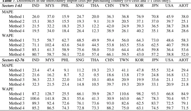
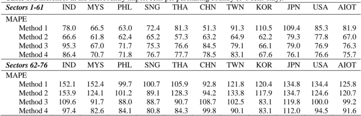
In all cases we will use the mean absolute deviation (MAD) and the mean absolute percentage error (MAPE) or the weighted absolute percentage error (WAPE) between our non-survey results and the semi-survey AIOT (IDE, 2006). We do not use squared errors as these give an unduly large weight to small errors (see Lahr, 2001, for a further discussion).8 For MAPE and WAPE, all cell-to-cell percentage differences and the weights are calculated using the average of the corresponding cell in the IDE table and the non-survey table. This has been done to cope with the large number of cases in which one of the two cells has a value of a zero. Please note that this has the important implication that the percentage error p between two cells a and b is defined as 200% for any pair of a and b for which one of the two values is zero, because p = 100 * |a-b| / 0.5(a+b). We will return to this issue in the next section.
5.1 Comparison at the domestic level: cells versus multipliers
For the domestic block-diagonal sub-matrices of the AIOT, a comparison of our non-survey tables with the IDE table is only relevant for Method 1. The mean absolute differences, which are measured in millions of US$, are of course largest for the larger economies of the USA and Japan (see Table 3). The last column gives the errors for the total of all domestic sub-matrices. The weighted percentage differences are significantly smaller than the unweighted ones, indicating that the larger percentage differences are found in the smaller cells of the IO tables, which is fine. For Singapore, Malaysia, Thailand and Taiwan the weighted errors should be considered large. For the other countries the differences seem acceptable.
When the import matrix is derived by using import ratios, as is done in Method 1, its “substitutability” with the survey-based import matrix depends on how similar the distribution patterns are between domestic products and imported products. For the large countries like China and the USA, which are quite self-sufficient and have a full-fledged type of industrial structure, the distribution patterns of imported items are considered to be similar to those of domestic products, and hence the separation of import matrix by simply using import ratios may be justified for producing non- survey tables. This is seen in the lower percentage errors for China and the USA in Table 3.
On the other hand, for the countries as Singapore and Malaysia which show high degree of specialisation in their industrial structure, it is less likely that the imported items are similarly produced by domestic industries, and hence the distribution patterns should be quite different between import and domestic products, giving poor results in the comparison between the non-survey table and semi-survey table.9
8 We do not use Lahr’s preferred measure, the weighted absolute difference (WAD), as taking absolute differences already takes the size of the cells into account.
9 For the discussion of specialisation of industrial structure, see Meng et al. (2006).
Table 3. Differences in the domestic cell values with Method 1.
IND MYS PHL SNG THA CHN TWN KOR JPN USA AIOT MAD 1.9 3.1 0.4 4.6 4.5 10.2 7.5 10.7 31.9 41.5 11.6 MAPE 19.6 32.9 5.7 32.3 26.1 5.5 24.9 18.3 10.1 7.8 18.3 WAPE 4.4 11.4 2.1 14.5 11.1 1.7 8.9 5.9 2.5 1.6 4.7
Table 4 gives a measure of holistic accuracy in that it indicates whether the positive and negative deviations in cell values compensate each other, as the percentage errors in the value added multipliers are only comparable with the errors in the IO cell values if these would all have the same sign. Table 4 shows that this is not the case. Except for Singapore, the percentage errors in the multipliers are rather small, indicating that positive and negative deviations in the estimation of the domestic IO cells compensate each other to a considerable extent. Besides, the MADs show that a 1000$ change in final demand produces errors in the estimate of the economy-wide value added effect of 8$ in the USA to 29$ in Thailand when Method 1 is used to estimate the domestic transactions. Thus, from a holistic point of view, the difference between the domestic parts of the first non-survey table and the semi-survey IDE table may be considered small, except for Singapore.
Table 4. Differences in domestic value added multipliers with Method 1.
IND MYS PHL SNG THA CHN TWN KOR JPN USA
MAD 0.022 0.024 0.008 0.023 0.029 0.018 0.025 0.027 0.016 0.008
MAPE 3.4 5.9 4.3 20.3 6.5 2.5 5.4 5.7 2.1 2.8
5.2. Comparison at the intercountry IO cell level
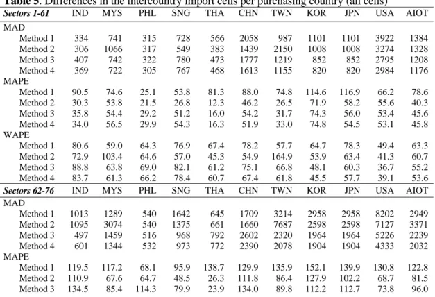
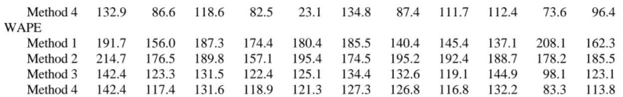
In Table 5 a comparison between the intercountry cells of the non-survey tables and the IDE table is made. As the non-service sectors 1-61 are treated differently than the service sectors 62-76, the results are given for both groups separately, with the MAD now measured in thousands of US$. The last column gives the errors for the whole intercountry part of the non-survey AIOT.
Table 5. Differences in the intercountry import cells per purchasing country (all cells)
Sectors 1-61 IND MYS PHL SNG THA CHN TWN KOR JPN USA AIOT
MAD
Method 1 334 741 315 728 566 2058 987 1101 1101 3922 1384 Method 2 306 1066 317 549 383 1439 2150 1008 1008 3274 1328 Method 3 407 742 322 780 473 1777 1219 852 852 2795 1208 Method 4 369 722 305 767 468 1613 1155 820 820 2984 1176
MAPE
Method 1 90.5 74.6 25.1 53.8 81.3 88.0 74.8 114.6 116.9 66.2 78.6 Method 2 30.3 53.8 21.5 26.8 12.3 46.2 26.5 71.9 58.2 55.6 40.3 Method 3 35.8 54.4 29.2 51.2 16.0 54.2 31.7 74.3 56.0 53.4 45.6 Method 4 34.0 56.5 29.9 54.3 16.3 51.9 33.0 74.8 54.5 53.1 45.8
WAPE
Method 1 80.6 59.0 64.3 76.9 67.4 78.2 57.7 64.7 78.3 49.4 63.3 Method 2 72.9 103.4 64.6 57.0 45.3 54.9 164.9 53.9 63.4 41.3 60.7 Method 3 88.8 63.8 69.0 82.1 61.2 75.1 66.8 48.1 60.3 36.7 55.2 Method 4 83.7 61.3 66.2 78.4 60.7 67.4 61.8 45.5 57.7 39.1 53.6
Sectors 62-76 IND MYS PHL SNG THA CHN TWN KOR JPN USA AIOT
MAD
Method 1 1013 1289 540 1642 645 1709 3214 2958 2958 8202 2949 Method 2 1095 3074 540 1375 661 1660 7687 2598 2598 7127 3371 Method 3 497 1459 516 968 792 2602 2320 1964 1964 5226 2239 Method 4 601 1344 532 973 772 2390 2078 1904 1904 4333 2032
MAPE
Method 1 119.5 117.2 68.1 95.9 138.7 129.9 135.9 152.1 139.9 130.8 122.8 Method 2 110.9 67.6 64.7 48.5 26.3 111.8 86.4 127.9 102.2 68.7 81.5 Method 3 134.5 85.4 114.3 79.9 23.9 134.0 89.8 112.2 112.7 73.8 96.0