A computational study on the generation of the Coanda effect in a mock heart chamber (Mathematical Analysis of Viscous Incompressible Fluid)

全文

(1)27. 数理解析研究所講究録第2009巻 2016年 27-43. A. computational study in A.. a. the generation of the Coanda effect mock heart chamber. Quainia. on. *. R.. Glowinskib and S. Čanic. aDepartment of Mathematics, University of Houston, Houston, TX 77204, USA bDepartment of Mathematics, Hong‐Kong Baptist University, Hong‐Kong. Abstract We present a numerical study of laminar incompressible flows in two‐dimensional and three‐dimensional contraction‐expansion channels. The aim is to understand the causes of the so‐called Coanda effect. order to. diagnosis. (i.e.,. the. in. a. fluid. jet. to be attracted to. (also. known. computations against the values found considered flow in. a. a. a. mock heart chamber constructed to. reproduce wall‐hugging jets of mitral valve regurgitation. First,. the onset of the Coanda effect we. of. tendency. surface). in. improve the. we validate the critical Reynolds number for symmetry‐Ureaking bifurcation) given by our literature. Excellent agreement is found. Then, heart chamber and showed how a pronounced. as. in the. section of the mock. Coanda effect is possible only with some modifications of the contraction channel geometry. Finally, we propose a 3\mathrm{D} mock heart chamber in which quasi‐2D flow is possible, thereby allowing the Coanda effect at the low Reynolds numbers for which it is observed in 2\mathrm{D}.. Introduction. 1. as the tendency nearby surface [27, 29], see Figure 1. The principle was named after Romanian aerodynamics pioneer Henri Coanda, who was the first to recognize the practical application of the phenomenon in aircraft development.. Coanda effect is. of. a. fluid. Figure. jet. 1:. a. phenomenon. to be attracted to. that is described in the scientific literature a. Steady state solution for The jet hugs the upper. Re=133.3. .. flow in. a. sudden. wall of the. expansion with expansion chamber.. a. 1. :. 6. expansion. at. Most recently, Coanda effect became popular in cardiology where it has been used to explain the wall hugging jets in certain cases of mitral valve regurgitation. Mitral regurgi‐ tation (MR) is a valvular disease characterized by abnormal leaking of blood through the mitral valve from the left ventricle into the left atrium of the heart. MR. can. lead to atrial. arrhythmias, pulmonary artery hypertension, congestive heart failure, and death. Diagnosis of mitral regurgitation is often performed using color Doppler echocardiography. Figure 2(a) shows the echocardiographic image of a jet flowing in the center of the left atrium (central jet), while Figure 2(b) shows the echocardiographic image of a jet hugging the wall of the left atrium. (eccentric jet),. Corresponding. known. author. Email:. as. the Coanda effect.. [email protected].

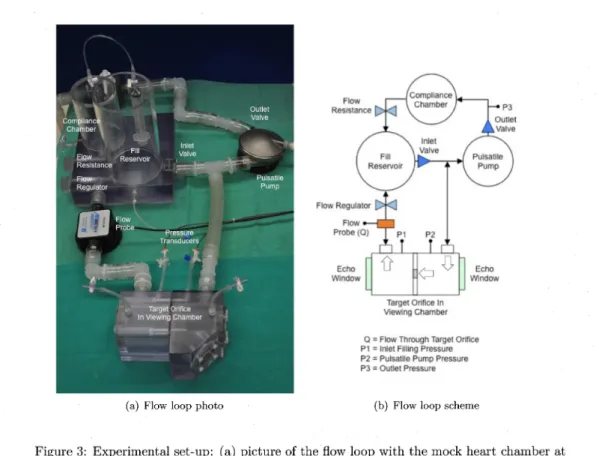
(2) 28. (a). Central color. Doppler jet. (b). Eccentric color. Doppler jet. Figure 2: (a) Echocardiographic image of central regurgitant jet flowing from the left ventricle (LV) to the left atrium (LA). Colors denote different flow velocities. (b) Echocardiographic image of eccentric regurgitant jet, hugging the walls of the left atrium (LA) known as the Coanda effect.. echocardiographic assessment of mitral regurgitation is hugs the wall of the hearts atrium as shown in 2 of the severity of MR is contaminated [9, the assessment Figure echocardiographic (b), 24]. These eccentric, wall‐hugging, non‐symmetric regurgitant jets that have been observed at Reynolds numbers well below turbulence [28, 1], appear smaller in the color Doppler image of regurgitant flow (due to the presence of a large secondary vortex), leading to a gross under‐estimation of regurgitant volume by inexperienced observers [9, 3]. As a result, patients who may require surgery are left untreated. Understanding the flow conditions and regurgitant orifice geometries responsible for the Coanda effect has been recognized to be of great importance for echocardiographic assessment of mitral valve regurgitation [9]. In our previous works [19, 20, 18], we showed that, once validated, a computational model provides detailed, point‐wise information about the quantities that are used in echocardio‐ graphic assessment of MR, thereby providing information that can be used to tune and refine the already existing protocols, or design new protocols. Our computational fluid model has been validated against experiments performed in an in vitro mock heart chamber shown in Figure 3. The mock heart chamber has been developed by our collaborators at the Methodist DeBakey Heart & Vascular Center [1e] to study 2\mathrm{D} and 3\mathrm{D} color Doppler techniques that are routinely used to image the complex intra‐cardiac flows associated with central MR jets [10, 11]. The chamber is composed of two acrylic cylinders partitioned by a divider plate containing a geometric orifice mimicking a leaky mitral valve and it was studied in a variety of clinically relevant flow conditions. However, our collaborators have never been able to reproduce in vitro the wall‐hugging MR jets typical of the Coanda effect. Despite of the large cardiovascular and bioengineering literature reporting on the Coanda effect in echocardiographic assessment of mitral regurgitation, there is very little connection with the fluid dynamics literature that could help identify and understand the main features of the corresponding flow conditions. In this paper, our goal is to understand what causes the onset of the Coanda effect in a simplified setting. A mitral regurgitant jet flows from the left ventricle through an orifice between the mitral leaflets, called regurgitant orifice, into the left atrium. As a simplified setting, which has the same geometric features as MR, we consider contraction‐expansion channels. First, we focus on the planar case (see Fig. 4(\mathrm{a}) ) and investigate the influence of the Reynolds number defined in eq. (6) and the expansion ratio $\lambda$=W/w where W and w are defined in Fig. 4(a). Then, we consider a 2\mathrm{D} geometry corresponding to a section of the mock heart chamber (see Fig. 8) in order to understand the role played by certain geometric features on triggering the Coanda effect. Finally, we will One of the. biggest challenges. in. Coanda effect: when the regurgitant jet. ,.

(3) 29. Target Orifice In v|\mathrm{e}\mathrm{w}| $\eta$ chatnber \mathrm{Q}\simeq FIow Th rough Targel Orfce. Pt. =. lnlet. Filllng. Pressure. \mathrm{P}2= Pulsatile Pump Pressure \mathrm{P}3\simeq OutDet Pressure. (a). Figure. 3:. Flow. (b). loop photo. Flow. loop. scheme. Experimental set‐up: (a) picture of the flow loop with the mock heart chamber picture and (b) its schematic representation.. at. the bottom of the. a 3\mathrm{D} mock heart chamber geometry in which the Coanda effect can be reproduced explain why it is unlikely to observe such an effect in the chamber currently used to simulate regurgitant flow in mitral valve regurgitation, shown in Fig. 3(a). The outline of the paper is as follows. In Section 2 we state the problem, discuss the. propose. and. numerical methods used for the time and space discretization and describe the solution of the associated linear system. In Section 3, we report on the results of the validation against [15] and [6]. In Section 4, we discuss the results for the flow in the mock heart chamber.. Finally, 2. conclusions. are. Numerical. drawn in Section 5.. modeling. The fluid in the mock heart chamber is water with 30% glycerin added to mimic blood viscosity (0.035 poise). The motion of such a fluid, which is incompressible, viscous, and Newtonian, in a spatial domain of dimension d (denoted hereafter by $\Omega$ ) over a time interval of interest (0, T) is described by the incompressible Navier‐Stokes equations:. $\rho$(\displaystyle \frac{\partial u}{\partial t}+u\cdot\nabla u)-\nabla\cdot $\sigma$=0 \mathrm{i}\mathrm{n} $\Omega$\times(0, T). \nabla\cdot u=0 \mathrm{i}\mathrm{n} $\Omega$\times(0, T) where $\rho$ is the fluid density, u is the fluid velocity, and Newtonian fluids, $\sigma$ has the following expression. $\sigma$(u,p)=-p\mathrm{I}+2 $\mu \epsilon$(u). $\sigma$. ,. the. Cauchy. ,. ,. stress tensor.. (1) (2) For.

(4) 30. where p is the pressure, $\mu$ is the fluid. dynamic viscosity,. and. $\epsilon$(u)=\displaystyle \frac{1}{2}(\nabla u+(\nabla u)^{T}) (1) -(2). is the strain rate tensor. In eq.. that. supposed. it is. ,. no. body. force is. applied. to the. system.. Equations (1) -(2). need to be. supplemented. with initial and. u=u_{D} \mathrm{o}\mathrm{n}\partial$\Omega$_{D}\times(0, T) $\sigma$ n=g \mathrm{o}\mathrm{n}\partial$\Omega$_{N}\times(0, T) in $\Omega$\times\{0\} u=u_{0}. conditions:. boundary. (3) (4) (5). ,. ,. .. \overline{\partial$\Omega$_{D} \cup\overline{\partial$\Omega$_{N} =\overline{\partial $\Omega$}. Here. and. \partial$\Omega$_{D}\cap\partial$\Omega$_{N}=\emptyset. under consideration g and u_{0} in Sections 3 and 4. the test. The. cases. number Re. Reynolds. In addition u_{D}, g and u_{0}. .. be used to characterize the flow. can. Re=\displaystyle\frac{$\rho$LU}{$\mu$} where L is can. be. characteristic. a. thought of as. inertial forces. length over. It is defined. as:. (6). ,. characteristic. a. regime.. velocity.. the ratio of inertial forces to viscous forces. For. dominant. are. and U is. given. For all as specified. are. set to zero, while u_{D} will vary. are. viscous forces and vice. The Reynolds number large Reynolds numbers. versa.. be seen as the limiting case of a reported Fig. 4(a) Fig. 4(b) for channel depth H tending to infinity. For the length L is given by the hydraulic diameter of the contraction. The flow in the 2\mathrm{D} geometry 3\mathrm{D} flow in the domain shown in 3\mathrm{D} problem, the characteristic channel, i.e. L=2Hw/(H+w). ,. in. (6). thus. can. becomes:. Re_{3D}=\displaystyle \frac{ $\rho$ U}{ $\mu$}\frac{2Hw}{H+w} By letting. (7),. H\rightarrow\infty in eq.. we. define the. Reynolds. Re=2\displaystyle \frac{ $\rho$ Uw}{ $\mu$} We define Re. as. (S). in. for the 2\mathrm{D} simulations U in. (8),. we. (7). .. number for the 2\mathrm{D}. problem. (8). .. with the purpose of comparing our results with [15] in Sec. 3 and section of the mock heart chamber. As characteristic velocity. on a. take the average velocity in the contraction channel. So, if we denote by U_{\max} velocity in the contraction channel and assume that the contraction channel. the maximum is. to have. long enough. a. fully developed parabolic velocity profile,. For the 3\mathrm{D} simulations in Sec. 4.2. (7),. take. we. will. use. definition. (7).. we. have. U=2U_{\max}/3.. As characteristic. velocity. U. the average velocity in the contraction channel. If we assume that in the contraction channel we have a fully developed parabolic velocity profile with maximum in. we. velocity U_{\max}. ,. again. this. U=U_{\max}/2.. means. problem (1) -(2). For the variational formulation of the fluid space of square. functions in. L^{2}( $\Omega$). inner. integrable. L^{2}( $\Omega$). functions in. a. spatial. with first derivatives in. product. and. a. duality pairing. L^{2}( $\Omega$). in $\Omega$ ,. ,. we. domain $\Omega$ and with .. We. use. )_{ $\Omega$}. denote. H^{1}( $\Omega$). and. respectively. Moreover,. let. by. L^{2}( $\Omega$). the. the space of the \}_{ $\Omega$} to denote the us. define:. [H_{D}^{1}( $\Omega$)]^{d}=\{v\in[H^{1}( $\Omega$)]^{d}, v|_{\partial$\Omega$_{D} =u_{D}\}, [H_{0D}^{1}( $\Omega$)]^{d}=\{v\in[H^{1}( $\Omega$)]^{d}, v|_{\partial$\Omega$_{D} =0\}, where. \partial$\Omega$_{D} is the part of the domain boundary. on. which. a. Dirichlet condition. (3). is. imposed..

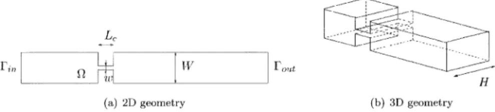
(5) 31. 6^{\sim_$zeta-}r{\mhf}_-aprox^{\ve-sim}^{<\ sim}-4_{\ sim-}\ acute{mhr}_\{sim-wedg^{}\simqpre.-\wdg^{vesim}\ prime-\s im-[_{}\rghtaowve\prim^{ghtaow\ve}mathr{J\piewdg\smipre'. \underline{L}_{c}. H. (a). Figure limit. 4:. case. (a). 2\mathrm{D} and. (b). 2\mathrm{D} geometry. (b). 3\mathrm{D}. (b). (a). is the. for H\rightarrow\infty.. The variational formulation of the fluid. [H_{D}^{1}( $\Omega$)]^{d}\times L^{2}( $\Omega$). The 2\mathrm{D} channel in. contraction‐expansion channel.. of the 3\mathrm{D} channel in. 3\mathrm{D} geometry. problem (1) -(2). is:. given t\in(0, T) find (u,p)\in ,. such that. $\rho$(\displaystyle \frac{\partial u}{\partial t}, v)_{ $\Omega$}+\mathcal{N}(u;[u,p], [v, q])_{ $\Omega$}=0, \foral (v, q)\in[H_{0D}^{1}( $\Omega$)]^{d}\times L^{2}( $\Omega$). (9). ,. with. \displaystyle \mathcal{N}(u;[u,p], [v, q])_{ $\Omega$}=2 $\mu$( $\epsilon$(u), $\epsilon$(v) _{ $\Omega$}+ $\rho$\int_{ $\Omega$}(u\cdot\nabla u)\cdot v\mathrm{d} $\Omega$-(p, \nabla\cdot v)_{ $\Omega$} +(\nabla\cdot u, q)_{ $\Omega$}. The initial condition is the. case. (10). .. given by (5). Notice that for. eq.. (9). we. assumed. g=0. in. (4). as. is. for the numerical tests in Sections 3 and 4.. Discretization. 2.1. equations (1) -(2) we chose the Backward Differentiation For‐ N_{T} [21]). Given \triangle t\in \mathbb{R} let us set t^{n}=t_{0}+n\triangle t with n=0, T=t_{0}+N_{T}\triangle t Problem (1) -(2) discretized in time reads: given u^{n} for n\geq 0, find the. For the time discretization of. (BDF2,. mula of order 2 and. see. ,. ,. .. solution. ,. (u^{n+1},p^{n+1}). $\rho$\displaystyle \frac{3u^{n+1}-4u^{n}+u^{n-1} {2\triangle t}+ $\rho$ u^{n+1}\cdot\nabla u^{n+1}-\nabla\cdot $\sigma$(u^{n+1},p^{n+1})=0. \nabla\cdot u^{n+1}=0. All the numerical test in Sections 3 and 4 in. (5). Thus,. we. take. For the space. of $\Omega$ made up of. are. \mathrm{i}\mathrm{n} $\Omega$ ,. (11). \mathrm{i}\mathrm{n} $\Omega$. (12). started from fluid at rest, that is. we. .. set. u_{0}=0. u^{-1}=u^{0}=0.. discretization, a. \backslash. of the system:. we. introduce. a. conformal and. (triangles. certain number of elements. quasi‐uniform partition T_{h}. in 2\mathrm{D} , tetrahedra in 3\mathrm{D} ). Let. V_{h}\subset[H^{1}( $\Omega$)]^{d}, V_{D,h}\subset[H_{D}^{1}( $\Omega$)]^{d}, Q_{h}\subset L^{2}( $\Omega$) be the finite element spaces approximating [H^{1}( $\Omega$)]^{d}, [H_{D}^{1}( $\Omega$)]^{d} and L^{2}( $\Omega$) respectively. We introduce the Lagrange basis \{$\phi$_{i}\}_{i=1}^{\mathcal{N}_{v} and ,. \{$\pi$_{i}\}_{i=1}^{\mathcal{N}_{p}. ,. V_{h} and Q_{h} (respectively), where \mathcal{N}_{v} is the number of nodes for the velocity approximation and \mathcal{N}_{p} is number of nodes for the pressure approximation. In order to write the matrix version of the fully discretized problem, we set: associated to. M_{i,j}=\displaystyle \int_{ $\Omega$} $\rho \phi$_{j}$\phi$_{i}.. ‐. The. ‐. The stiffness matrix:. ‐. ‐. mass. matrix:. K_{i,j}=2\displaystyle \int_{ $\Omega$} $\mu \epsilon$($\phi$_{j}): $\epsilon$($\phi$_{i}). The matrix associated with the convective term: The matrix associated with operator. (-\nabla:). :. .. N_{i,j}(u^{n+1})=\displaystyle \int_{ $\Omega$} $\rho$(u^{n+1}\cdot\nabla)$\phi$_{j}\cdot$\phi$_{i}.. B_{i,j}=-\displaystyle \int_{ $\Omega$}(\nabla\cdot$\phi$_{j})$\pi$_{i}..

(6) 32. The full discretization of. problem (1) -(2) yields. the. following. nonlinear. \displaystyle \frac{3}{2\triangle t}M\mathrm{U}^{n+1}+K\mathrm{U}^{n+1}+N(u^{n+1})\mathrm{U}^{n+1}+B^{T}\mathrm{P}^{n+1}=\mathrm{b}_{u}^{n+1}. B\mathrm{U}^{n+1}=\mathrm{b}_{p}^{n+1} \mathrm{U}^{n+1}. where. \mathrm{b}_{u}^{n+1}. and. and. \mathrm{b}_{p}^{n+1}. \mathrm{P}^{n+1}. are. (13). ,. (14). ,. the arrays of nodal values for. and pressure. The arrays previous time steps and. velocity. account for the contributions of the solution at the. the contribution that the. Set. system. boundary nodes give. C=\displaystyle \frac{3}{2\triangle t}M+K+N(u^{n+1}). .. We. can. to the internal nodes.. (13) -(14). rewrite. A\mathrm{X}^{n+1}=\mathrm{b}^{n+1}. in the form. (15). ,. where. A=\left\{ begin{ar ay}{l} C&B^{T}\ B&0 \end{ar ay}\right\},\mathrm{X}^{n+1}=\left\{ begin{ar ay}{l \mathrm{U}^{n+1}\ \mathrm{P}^{n+1} \end{ar ay}\right\},\mathrm{b}^{n+1}=[\mathrm{b}_{p}^{n+1}\mathrm{b}_{u}^{n+1}]. In order to deal with the convective term every. fixed‐point iteration,. we use a. to solve the linearized version of. nonlinearity, we use parallel sparse. a. system. fixed‐point algorithm.. direct solver. multifrontal. (see,. e.g.,. At. [5]). (15).. approximation of the incompressible Navier‐Stokes equations re‐ the pair (Q_{h}, V_{h}) does not satisfy the well‐known inf‐sup to be able to use equal order velocity‐pressure pairs (which condition are not inf‐sup stable, like the \mathbb{P}_{1}-\mathbb{P}_{1} finite elements we used for the results in this paper), The standard Galerkin. ported. we. in. (13)-(14) is unstable if (see, e.g. [22]). In order. resort to. a. stabilized formulation.. adopt is the orthogonal subgrid scales (OSS) technique proposed provides pressure stability and stabilizes the convective term for high [4]: Reynolds numbers. Let u_{h} and p_{h} be the space discrete velocity and pressure. The stabilized version of the problem under consideration reads: given t\in(0, T) find (u_{h},p_{h})\in V_{h}\times Q_{h} The stabilization method that in. we. it. ,. $\rho$(\displaystyle \frac{\partial u_{h} {\partial t}, v_{h})_{ $\Omega$}+\mathcal{N}_{s}(u_{h};[u_{h,Ph}], [v_{h}, q_{h}])_{ $\Omega$}=0, \foral (v_{h}, q_{h})\in V_{D,h}\times Q_{h}, where. \mathcal{N}(u_{h};[u_{h},p], [v_{h}, q_{h}])_{ $\Omega$}. in the discretization of. (9). has been. replaced by. \mathcal{N}_{s}(u_{h};[u_{h},p_{h}], [v_{h}, q_{h}])_{ $\Omega$}=\mathcal{N}(u_{h};[u_{h},p_{h}], [v_{h}, q_{h}])_{ $\Omega$} +S (u_{h};[u_{h},Ph][v_{h}, q_{h}])_{ $\Omega$}. The. perturbation. term S introduced. by OSS (in. quasi‐static form) reads. its. S (u_{h};[u_{h)}p_{h}], [v_{h}, q_{h}])_{ $\Omega$}=($\tau$_{1}$\Pi$^{\perp}(u_{h}\cdot\nabla u_{h}+\nabla p_{h}), u_{h}\cdot\nabla v_{h}+\nabla q_{h})_{ $\Omega$} +($\tau$_{2}$\Pi$^{\perp}(\nabla\cdot u_{h}), \nabla\cdot v_{h})_{ $\Omega$}. (16). .. L^{2} orthogonal projection onto the finite element space, i.e.: $\Pi$^{\perp} the iden‐ is the L^{2} projection onto the finite element space and \mathcal{I} tity operator. For the choice of the stabilization parameters $\tau$_{1} and $\tau$_{2} and for a thorough. Here, $\Pi$^{\perp}. is the. =. where $\Pi$. - $\Pi$. \mathcal{I}. technique, we refer to [4]. by C_{s} the sum of matrix C and the corresponding stabilization terms obtained from (16). Similarly, we denote by B_{s} ( B_{s}^{T} resp.) the sum of matrix B ( B^{T} resp.) and the corresponding stabilization terms. Moreover, we denote by L_{ $\tau$} the matrix associated with the pressure stabilization. The stabilized fully discrete problem can be written in matrix description Let. us. of this stabilization. denote. ,. form. (15). ,. as. A=\left\{ begin{ar y}{l C_{s}&B_{s}^{T}\ B_{s}&L_{$\tau$} \end{ar y}\right\},\mathrm{X}^{n+1}=\left\{ begin{ar y}{l \mathrm{U}^{n+1}\ \mathrm{P}^{n+1} \end{ar y}\right\})\mathrm{b}^{n+1}=\left\{ begin{ar y}{l \mathrm{b}_{u}^{n+1}\ \mathrm{b}_{p}^{n+1} \end{ar y}\right\}. For e.g.,. more. [22].. details. concerning. the discretization of the Navier‐Stokes. problem,. we. refer to,.

(7) 33. Preliminary study. 3. of. a. contraction‐expansion channel. against the results reported in [15] perform planar contraction‐expansion channels with [6]. two different values of the expansion ratio $\lambda$ to identify the critical Reynolds number Re_{sb} at which the jet ceases to be symmetric (i.e., central; see Fig. 2(\mathrm{a}) ) to become wall‐hugging (i.e., eccentric; see Fig. 2(\mathrm{b}) ). This is known in the literature as symmetry breaking bifurcation. Once our solver has been validated and convergence studies have been performed showing good convergence properties, it can be used as a predictive tool for discovery of new physical phenomena. The main aim of this section is to validate and. We. Let. us. a. our. solver. series of simulations in. start with the test. case. in. [15].. The. geometry under consideration is shown in. Fig. 4(a) with the upstream and downstream channel width W=4 , and contraction width w=0.26 Thus, the expansion ratio $\lambda$=W/w is 15.4. The length of the contraction L_{c} is .. set to 2. In this. domain,. we. simulate the flow for different. Reynolds. numbers. 71.3) to ,examine the onset of asymmetries. Eq. (1) -(2) are supplemented with the following steady boundary. (ranging. from. 0.01 to. velocity profile condition the. on. at the inlet. the rest. conditions:. parabolic. $\Gamma$_{in} stress‐free boundary condition at the outlet $\Gamma$_{out} and no‐slip of the boundary. Both the channel upstream of the contraction and. expansion channel need. ,. to be. ,. long enough. so. that the flow is. reaches the contraction and the outlet section. The fluid is. established when it. fully. at rest. A time. marching algorithm is used to approach the steady‐state solution. The numerical simulations were stopped when the relative L^{2} ‐norm of the difference of two subsequent solutions was less that a prescribed tolerance $\epsilon$ :. \displaystle\frac{|\mathrm{u}_h^{n+1}-\mathrm{u}_h^{n}|_{L^2}($\Omega$)}{|\mathrm{u}_h^{n+1}|_{L^2}($\Omega$)}\leq$\epsilon$. and. initially. \displayst le\frac{|p_{h}^{n+1}-p_{h}^{n}|_{L^2}($\Omega$)}{|p_{h}^{n+1}|_{L^2}($\Omega$)}\leq$\epsilon$. ,. (17). \mathrm{u}_{h}^{n+1} (resp., \mathrm{u}_{h}^{n} ) and p_{h}^{n+1} (resp., p_{h}^{n} ) are the computed velocity and pressure at time t^{n+1} (resp., t^{n} ). The value of $\epsilon$ was set to 10^{-8}. In Fig. 5, we report the streamlines at the time when stopping criterion (17) is satisfied for four different values of Re. For very low Reynolds number (e.g., Re =0.01 ), it is impossible to deduce the flow direction from the streamlines: as shown in Fig. 5(a), the flow has both a horizontal and vertical symmetry axis. As the Reynolds number is increased, the Moffatt eddies (see [14]) downstream of the expansion grow while the vortices upstream of the contraction reduce in size: we see in Fig. 5(b) that the flow at Re=7.8 has lost the symmetry about the vertical axis, while the symmetry about the horizontal axis is maintained. At a further increase of the Reynolds number, the flow becomes asymmetric also with respect to the horizontal symmetry axis of the domain; see Fig. 5(c) which corresponds to Re=31.1 In Fig. 5(c), the lower recirculation enlarged and pushed the high velocityjet to the upper wall. Notice that the flow could have evolved to its reflected image configuration with respect to the domain symmetry axis. A further increase in Reynolds number generates a third vortex downstream on the side of the smaller primary vortex, as the enlarged one grows and pushes the jet even closer to the wall; see Fig. 5(d). Fig. 5 is in good qualitative agreement with where. .. [15]. It. shown. [26, 8, 25, 13]. that this behavior. result of. supercritical pitchfork Re_{sb} two stable solutions equations, i.e., co‐exist [2]. Bifurcation theory allows to clarify the nature of the multiplicity of possible flows, whereas \mathrm{a} (numerical or laboratory) experiment will give one or the other of the stable asymmetric solutions. The asymmetric solution remains stable for a certain range of Re and asymmetries become stronger with the increasing Reynolds number, as shown in [12]. The formation of stable asymmetric vortices in 2\mathrm{D} planar expansion is due to the Coanda effect (see [29]): an increase in velocity near one wall will lead to a decrease in pressure near was. occurs as a. bifurcation in the solution of the Navier Stokes. that wall and. once a. pressure difference is established. a. above. across. the channel it will maintain the.

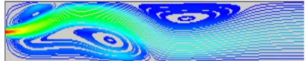
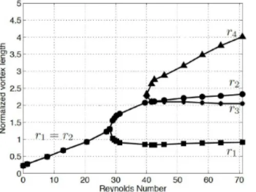
(8) 34. (a). (b). Re=0.01. (c). Re=7.8. \rightarrow. Re=31.1. r_{4}. \rightarrow r_{3} r_{1}. r_{2}. (d). Re=71.3. Figure 5: Expansion ratio $\lambda$=15.4 : Streamlines at the time when stopping criterion (17) is satisfied for Reynolds numbers (a) Re=0.01 (b) Re=7.8 (c) Re=31.1 (d) Re=71.3. The streamlines are colored with the velocity magnitude, with blue corresponding to 0 and red corresponding to 1. ,. ,. ,. asymmetry of the flow. The value of Re_{sb} has been identified for different expansion ratios $\lambda$ In particular, it was found that Re_{sb} decreases with increasing value of $\lambda$ (see [6, 23, 13 For a quantitative agreement, we report the bifurcation diagram shown in Fig. 6, which .. Reynolds number on the length of the recirculation zones formed expansion and it is identical to the one presented in [15]. The lengths in Fig. 6 ( r_{1} to r_{4} as marked in Fig. 5(\mathrm{d}) ) are normalized with respect to the downstream channel width W As in [15], the critical Reynolds number for the symmetry breaking Re_{sb} was found to be approximately 28.5, which is in good agreement also with the results in [12]. In fact, reference [12] considers $\lambda$=16 and obtains a critical Reynolds number of 27.5, which is very close to what we get. At Re between 41 and 42, the third vortex appears. shows the effect of the. downstream of the ,. .. Figure. 4(\mathrm{a}). 6:. Expansion. ratio $\lambda$=15.4 :. bifurcation. diagram. for the geometry shown in. Fig.. .. For. further validation of the. results,. consider. from. [6].. Since. only expansion varies, going to consider the domain reported in Fig. 7(a): the inlet $\Gamma$_{in} of this new geometry is the outlet of the contraction channel in Fig. 4(a). The expansion chamber width W is set to 1 and a. we. interested in the evolution of the vortices in the. a. test. case. channel. as. Re. we are. we are.

(9) 35. |\mathrm{I}_ $\lambda$J/}. (l.| -\mathrm{b}. (a) Geometry. considered in. [6]. (b). Bifurcation. diagram. for $\lambda$=6. Figure 7: (a) Computational geometry considered in [6] and (b) a convergence study for the bifurcation diagram corresponding to the 2\mathrm{D} flow in such geometry with $\lambda$=6 The results refer to three different meshes: coarse, medium, and fine. .. the contraction width. 1/6,. implies $\lambda$=6 This is one of the geometries length L_{c} (see Fig. 4) is large enough to have an established Poiseuille flow in it, the flow upstream of the contraction is not going to affect the flow downstream. In this domain, we examine the onset of asymmetries by simulating the flow for Reynolds numbers ranging from 0.01 to 73.3. As boundary conditions, we impose a parabolic velocity profile with maximum velocity U_{\max}=1 on $\Gamma$_{in} a stress‐free boundary condition at the outlet $\Gamma$_{out} and no‐slip condition on the rest of the boundary. We change the Reynolds number by varying the value of the viscosity $\mu$ The stopping tolerance for the fixed point iterations was set to 10^{-8} since as considered in. [6].. is. w. equal. to. which. .. Note that if the contraction channel. ,. ,. .. the. ,. Reynolds. number increases the convective term needs to be. For this second test case,. we. checked the influence of the mesh size. Three meshes with different levels of refinement ‐. a coarse. diameter. ‐. mesh, with. an. has around. 10^{4} nodes and. medium. with. a. mesh,. and. a. a. fine. mesh,. around 4.4. \cdot. with. Re_{sb}.. ,. a. maximum element. h_{\min}=10^{-2} ;. this mesh. triangles;. h_{avg}=1.3\cdot 10^{-2}, h_{\max}=2.8\cdot 10^{-2}, h_{\min}=5\cdot 10^{-3} ;. this mesh has. was. traction. The bifurcation. length of. the value of. this mesh has. 10^{4} nodes and 8.7. The minimum diameter. on. h_{avg}=2.3\cdot 10^{-2}, h_{\max}=4\cdot 10^{-2}, h_{\min}=7\cdot 10^{-3} ;. around 2. 2\cdot 10^{4} nodes and 4. 3\cdot 10^{4} ‐. h_{avg}=4\cdot 10^{-2}. minimum element diameter. 1. 9\cdot 10^{4}. resolved.. considered:. were. average element diameter. h_{\max}=6\cdot 10^{-2}. properly. the recirculation. \cdot. triangles;. 10^{4} triangles.. set at the inlet in order to have proper resolution of the. diagram Fig. 7(b) regions. Since now W=1 in. shows the effect of ,. number. con‐. the Reynolds lengths correspond to on. the normalized. the actual. lengths. Fig. 7(b) we see that for $\lambda$=6 the third recirculation does not appear for Re\leq 73.3, regardless of the mesh used, while for $\lambda$=15.4 it appeared just past Re=41 We observe that the results for the medium mesh and the fine mesh are almost superimposed and they both give a value of Re_{sb} approximately equal to 46.5. Notice that as the aspect ratio $\lambda$ decreases, the critical Reynolds number for the symmetry breaking increases, as observed also in [6]. The bifurcation graph in Fig. 7(b) is very similar to the one in [6], taking into account the fact that we defined the Reynolds number as in (8) with the characteristic velocity U=2U_{\max}/3 while in [6] the Reynolds number is defined as in (6) with L=w and U=U_{\max}, U_{\max} being the maximum inlet velocity. Converting our value Re,b=46.5 to the system used in [6] we get 34.8, which is very close to 33, the value found in [6]. Fig. 7(b) From. .. ,.

(10) 36. computations are performed on a mesh that is under‐refined, the value of Re_{sb} gets overestimated. At larger Reynolds number the flow becomes increasingly complex and other bifurcations occur. At a further increase of Re, the flow becomes unsteady and the existence of a Hopf bifurcation is deduced [26]. In [17], for $\lambda$=6 we showed that a Hopf bifurcation does occur in the expansion channel: at a certain Reynolds number the asymmetric solution loses its stability and a one‐parameter family of periodic solutions bifurcates from the stationary shows that if the. solution.. Numerical results for the mock heart chamber. 4. In this. study. section,. sheds. construct. shown in. light. on. the. causes. section of the mock heart chamber. This 2\mathrm{D}. a. of the Coanda effect and. helps. 3\mathrm{D} mock heart chamber in which the Coanda effect. comment. we. on. why. it is. unlikely. to observe such. an. us. be. can. understand how to. reproduced. Finally,. effect in the current mock heart chamber. Fig. 3(a).. A section of the chamber. 4.1 Let in. a. first consider the flow in. we. some. us. consider the radial section of the real chamber. Fig. 3(a). The geometry of this. ratio $\lambda$=45. Fig. 4(a).. .. section is. a. parallel to the horizontal chamber walls contraction‐expansion channel with expansion. Notice that the inlet and outlet sections for this channel differ from those in. through two tubes whose changed inlet and outlet with respect to the channels in the previous section to reflect the flow configuration in the real chamber. Based on the results reported in Sec. 3, we expect the wall‐hugging effect to appear at a very low Reynolds number since the channel under consideration has $\lambda$=45 In Fig. 8, we report the streamlines at the time when stopping criterion (17) is satisfied for three different values of Re. For a Reynolds number equal to 2, the jet expands in the center of the expansion chamber as shown in Fig. 8(a). Notice that due to the modified inlet and outlet sections, we cannot refer to the jet in Fig. 8(a) as symmetric, however there is clearly no wall‐hugging effect taking place. As the Reynolds number is increased to 20, the upper downstream recirculation zone becomes bigger than the lower recirculation: the jet is pulled towards the outlet, yet again no Coanda effect is displayed; see Fig. 8(b). At Re=100 instead, the jet hugs the lower wall before reaching the outlet as shown in Fig. 8(c). Moreover, from Re=20 to Re=100 secondary recirculations have appeared and the flow has become increasingly complex. In Sec. 3, we noted that if the contraction channel length L_{c} (see Fig. 4(\mathrm{a}) ) is large enough to have established Poiseuille flow in it, the flow upstream of the contraction is not going In. fact,. the fluid enters end exits the mock heart chamber. dimeter is smaller that the chamber diameter. We. .. to affect the flow downstream. In the. geometry under consideration the contraction channel. is very small because healthy mitral valve leaflets have a thickness of less than 5 For this reason, we decided to check whether different flows upstream of the contraction. length mm.. lead to different flows in the time when the. stopping. inlet at the left vertical wall. (i.e.,. as. Fig. 8). Fig.. in. expansion chamber. We report. criterion. (as. (17). in. Fig.. 9 the streamlines at the. is satisfied for Re=100 and two inlet. for the channels in Sec.. 9 shows that also for. a. 3). and inlet. as. configurations:. in the real chamber. short contraction channel. length. the flow. upstream of the contraction does not influence the flow in the expansion chamber. If the Reynolds number is further increased from 100 the solution becomes time‐dependent,. indicating not. that. a. Hopf bifurcation. has occurred.. Thus, increasing the Reynolds number. is. viable way to make the Coanda effect more pronounced. In the following, we are go‐ to consider a couple of geometry modifications that will push the jet to the wall almost a. ing throughout. its entire. length,. as. observed in vivo. (see Fig.. 2. (b))..

(11) 37. (a). (b). Re=2. (c). Figure 8: Streamlines. in. (a). (b). number:. Re=2 ,. (a) Large. a. Re=20. Re=100. section of the mock heart chamber for different values of. Re=20 , and. (c). Reynolds. Re=100.. Small horizontal inlet. (b). vertical inlet. Figure 9: Streamlines for Re=100 in a section of the mock heart chamber for two inlet configurations: (a) inlet at the left vertical wall and (b) inlet as in the real chamber. The arrows. indicate the flow direction.. The mitral valve is. a. bi‐leaflet valve. The anterior leaflet. of the total valve surface. See is. unlikely. (see Fig. 11(\mathrm{a}) ). prolapse, which. left atrium. This. to form in the center of the valve.. to the lower wall. valve. Fig. 10(a).. as. means. covers. approximately. two‐thirds. that the orifice between the leaflets. For this reason,. rather than in the center. we. consider. an. orifice closer. (see Fig. 8). Moreover, mitral. by the displacement of a mitral valve leaflet into the typically observed in patients with eccentric regurgitant geometry with an uneven orifice reported in Fig. ll(b).. is characterized. shown in. Fig. 10(b),. is. jets. Therefore we consider the Fig. ll(a) shows that when the orifice is closer to the lower wall the recirculation below the jet in the expansion chamber is smaller than in the case of a central orifice, so \mathrm{t}\mathrm{h}_{\mathrm{t}\mathrm{e} wall‐ hugging effect becomes more pronounced. Compare Fig. ll(a) with Fig. 9(a), which were both obtained for Re=100 In the case of an uneven orifice (i.e., prolapsed valve), the jet hugs the lower wall along its entire length. See Fig. ll(b), which also corresponds to .. Re=100. In summary, this 2\mathrm{D}. study. in. a. section of the real chamber indicates that. an. evident. be achieved thanks to two geometry modifications: lowering the location of the orifice (closer to the outlet), and making the orifice plate uneven. Next, we are going. Coanda effect. to. use. can. be. can. these conclusions to construct. reproduced.. a. 3\mathrm{D} mock heart chamber in which the Coanda effect.

(12) 38. (a). 10:. Figure. valve and. (a) Anatomy a. of the mitral valve. and. prolapse. (b) comparison. (b). Lower orifice. 11: Streamlines for Re=100 in. orifice. configurations: (a). 4.2. A 3\mathrm{D} chamber with. between. a. normal mitral. a. Uneven orifice. section of the mock heart chamber for two modified. lower orifice and. quasi‐2D. (b). uneven. orifice.. flow. Fig. 4(b) was considered and an extensive set of simulations was expansion ratio $\lambda$=14.5 and variable aspect ratio $\chi$=H/w The goal was to understand how the flow varies in a 3\mathrm{D} contraction‐expansion channel as the Reynolds number (defined in eq. (7)) and $\chi$ change. In. [15],. [16]. Mitral valve. prolapsed mitral valve.. (a). Figure. (b). Mitral valve anatomy. the 3\mathrm{D} channel in. carried out for. Let. us. .. introduce dimensionless variable. the values of \mathcal{H}. to the Hele‐Shaw flow. limit, and 1, for. $\chi$=0. $\chi$\rightarrow\infty which. corresponds. to the 2\mathrm{D} flow limit. It. Re_{3D} there is. no. ,. which. which. \mathcal{H}=H/(H+w)= $\chi$/( $\chi$+1) :. is bounded between 0 , for. an. was. found in. [15]. that for low \mathcal{H} and low. visible recirculation formed downstream of the. corresponds. to. expansion. For Re_{3D}>28.5, the critical value for the symmetry breaking in 2\mathrm{D} fo.r $\lambda$=14.5 the ,. sequence of events when \mathcal{H} varies is. irrotational flow.. channels. These. corresponds. as. follows. For low \mathcal{H}. (e.g., 0.01). the flow still resembles. As \mathcal{H}. vortices,. increases, small vortices form at the outlet of the contraction lip vortices form only in the three‐dimensional flow and the planar case. When \mathcal{H} reaches the value of 0.5, in addition to called. they are not observed in lip vortices, corner vortices appear. The latter are the Moffatt eddies observed also in the bi‐dimensional flow (see Fig. 5(\mathrm{a}) ). A further increase of \mathcal{H} leads to the formation of full corner recirculations as those in Fig. 5(b). Only for high values of \mathcal{H} (e.g., 0.8), asymmetric flow with large recirculations is observed. The results in [15] show that the vertical walls in Fig. 4(b) have a stabilizing effect on the flow patterns by inhibiting the onset of flow asymmetries, i.e. fully three‐dimensional flow prevents the flow asymmetries observed in quasi‐2D flow at the same Reynolds number. In fact, the results in [15] indicate that the asymmetric solution, corresponding to the Coanda effect, is obtained for larger Reynolds numbers and for channels with larger normalized depth \mathcal{H} Since \mathcal{H}=H/(H+w) where w is the width of the contraction channel and H is the depth, this implies that Coanda effect occurs for the contraction channels which are the. .. ,.

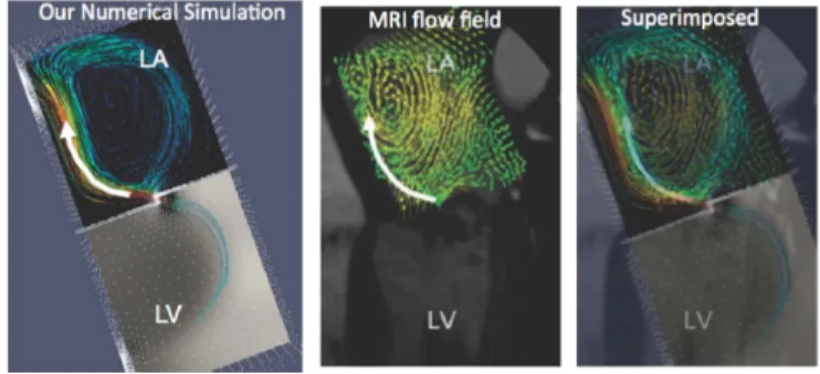
(13) 39. (w<<H). slender. .. This information. can. be related to the studies of Coanda effect in mitral. depth of the channel corresponds to the regurgitant orifice length, while the width of the channel corresponds to the orifice width. Therefore, the Coanda effect is expected to occur for regurgitant orifices which are long and narrow, i.e., for those for which. regurgitation:. the. w<<H. The mitral valve leaflets, when the valve is closed, make contact along a relatively long region, called coaptation. See Figure 12(a). In regurgitant valves when the two leaflets do not close properly, the length of the coaptation region that stays open corresponds to the depth in the contraction channel, denoted by H in Figure 12. Thus, in the case of mitral valve regurgitation, one can expect to see Coanda effect in cases when the regurgitation occurs along a large portion of the mitral coaptation and at larger Reynolds numbers.. and. (a). 12:. Figure. (b). Sketch of. sketch of. We test. our. an. a. regurgitant mitral valve, viewed from the top (left atrium) regurgitant jet in the magnified view of the valve in (a).. closed. eccentric. hypotheses by constructing. a. 3\mathrm{D} mock heart chamber with. a. slender orifice:. extrude the section of the real chamber considered in Sec. 4.1 to achieve aspect ratio $\chi$=45 , corresponding to \mathcal{H}=0.98 See Fig. 13. Notice in Fig. 13(b) that the extrusion. we. .. generates also elongated inlet and outlet sections.. (a). Figure. 13:. in Sec. 4.1.. 3\mathrm{D} chamber for. quasi‐2D. flow. \upar ow. \downar ow. |\mathrm{n}|\mathrm{e}\mathrm{t}. 0utlet. (b). Chamber skeleton. (a) 3\mathrm{D} chamber generated by extruding the section (b) Skeleton of the chamber in (a).. We report in. Fig.. 14 the streamlines at the time when. of the real chamber considered. stopping criterion (17). is satisfied. for Re_{3D}=100 and two orifice configurations: even and uneven orifice. In the case of the even orifice shown in Fig. 14(a), the big recirculation below the jet in the expansion chamber On the an evident wall‐hugging effect, as already observed in 2\mathrm{D} (see Fig. 8(\mathrm{c}) ). hand, the jet passed through the uneven orifice hugs the expansion chamber walls along its entire length, as shown in Fig. 14(b). Fig. 15 shows the velocity magnitude on the central vertical section of the geometry in Fig. 13(a) for both the even and the uneven orifice. Notice how closely the flow resembles the corresponding 2\mathrm{D} flow in Fig. 8(c) and 11(b), respectively. This shows that far away from. prevents. other. the vertical wall the flow does not feel the presence of the walls. This 3\mathrm{D} chamber succeeds.

(14) 40. (a). Figure. 14: Streamlines in the 3\mathrm{D} chamber shown in. Fig. 13(a). configurations: (a). (b). 100 and two orifice. in. (b). Even orifice. even. orifice and. producing quasi‐2D flow, thereby allowing. Uneven orifice. for. Reynolds. uneven. number Re_{3D}=. orifice.. the Coanda effect at the low. Reynolds. numbers. for which it is observed in 2\mathrm{D}.. (a). Figure 15: Velocity magnitude for two orifice. (b). Even orifice. on. configurations: (a). Uneven orifice. the central vertical section of the geometry in orifice and (b) uneven orifice.. Fig. 13(a). even. orifice, which corresponds to a prolapsed valve, we compared our numerical experimental data acquired by Magnetic Resonance Imaging in Fig. 16. The qualitative comparison is excellent. The 3\mathrm{D} chamber proposed in this section successfully recreates the Coanda effect because it allows for quasi‐2D flow since it is made of two cubes, it has elongated (rectangular) inflow and outflow sections, and a slender orifice. The real chamber shown in Fig. 3(a) is made of two cylinders, it has small (circular) inflow and outflow sections and a small orifice. Thus, the flow in the real chamber is fully 3\mathrm{D} inhibiting the onset of wall‐hugging jets. For this reason, it is unlikely to observe such an effect in the real mock heart chamber. For the. uneven. results with. ,. 5. Conclusions. presented a numerical study aimed at understanding the causes of the Coanda effect in contraction‐expansion channels. The dynamics of these systems were analyzed by means of direct numerical simulation of the unsteady NavierStokes equations. This was a first step towards establishing a connection between the large cardiovascular and bioengi‐ neering literature reporting on the Coanda effect in echocardiographic assessment of mitral regurgitation and the fluid dynamics literature. The long term goal of this work is to improve the diagnosis of mitral valve regurgitation for eccentric, wall‐hugging jets. In contraction‐expansion channels, a steady symmetric flow is observed for sufficiently small values of the Reynolds number. Above a certain critical Reynolds number, a steady asymmetric solution is observed: recirculation zones of different sizes form on the upper and lower wall. We validated the critical Reynolds number for the symmetry‐Ureaking bifurcation given by our computations against the value in [15] for expansion $\lambda$=15.4 and the value in We. 2\mathrm{D} and 3\mathrm{D}.

(15) 41. Figure 16: Qualitative comparison between our simulation of flow in the mock left atrium (LA) chamber and Magnetic Resonance Imaging of flow in LA [7]. The fluid is flowing from the left ventricle. [6]. for $\lambda$=6. Next,. .. we. (LV).. Flow streamlines. Excellent agreement. considered the flow in. was. a. are. shown.. found.. section of the mock heart chamber. our. medical collabo‐. hemodynamics encountered in patients with MR. Such a section is a 2\mathrm{D} contraction‐expansion channel with a large expansion ratio ( $\lambda$=45) Through a series of numerical simulations we show that a pronounced Coanda effect is possi‐ ble only with some modifications of the orifice (i.e., contraction channel) geometry. Thanks to these results and the results in 3\mathrm{D} contraction‐expansion channels reported in [15], we argue that in the real chamber the fully three‐dimensional flow prevents the wall‐hugging effect observed in 2\mathrm{D} flow at the same Reynolds number. Finally, we propose a 3\mathrm{D} mock heart chamber in which quasi‐2D flow is possible, thereby allowing the Coanda effect at the low Reynolds numbers for which it is observed in 2\mathrm{D}. rators. use. to. reproduce. in vitro the cardiac. .. Acknowledgements supported in part by the National Science Foundation under grants DMS‐1318763, DMS‐1311709, and DMS‐0806941 (Canic), DMS‐1263572 and DMS‐1109189 (Canic and Quaini), and by the Texas Higher Education Board (ARP‐Mathematics) 003652‐ This research has been. 0023‐2009. (Canic. and. Glowinski).. Hospital in Houston is gratefully acknowledged for the images pictures experimental set‐up. The authors would also like to thank Professor Hishida from University of Nagoya for giving them the opportunity to contribute to the proceedings of a most exciting Navier‐Stokes equations dedicated workshop. Dr. S. Little from the Methodist. medical. and the. of the. References. [1]. J. Albers, T. Nitsche, J. Boese, R. De Simone, I. Wolf, A. Schroeder, and. F. Vahl. Regurgitant jet evaluation using three‐dimensional echocardiography and magnetic res‐ onance. Ann Thorac Surg, 78:96−102, 2004.. [2]. F.. Battaglia, S.J. Tavener, A.K. Kulkarni, and C.L. Merkle. Bifurcation of low Reynolds symmetric channels. AIAA J., 35:99−105, 1997.. number flows in. [3]. K.. Chao, V.A. Moises,. the Coanda effect 1992.. on. R.. Shandas, T. Elkadi, D.J. Sahn, and R. Weintraub. Influence of Doppler jet area and color encoding. Circulation, 85:333−341,. color.

(16) 42. [4] [5]. R. Codina.. Stabilized finite element approximation of transient incompressible flows using orthogonal subscales. Comput. Methods Appl. Mech. Engrg., 191:4295−4321, 2002. T.A. David and I.S. Duff. An. unsymmetric‐pattern multifrontal method for Appl., 18(1):140-158 1997.. factorization. SIAM. J. Matrix Anal. ty. [6]. D. Drikakis.. Bifurcation. Fluids, 84:76−87,. phenomena. in. sparse LU. ,. incompressible sudden expansion flows. Phys.. 1978.. [7]. Dyverfeldt, J. Kvitting, C. C. 11, G. Boano, A. Sigfridsson, U. Hermansson, A. F. Bolger, J. Engvall, and T. Ebbers. Hemodynamic aspects of mitral regurgitation as‐ sessed by generalized phase‐contrast MRI. Journal of Magnetic Resonance Imaging, page 33:582588, 2011.. [8]. R.M.. P.. Fearn, T. Mullin, and K.A. Cliffe. Nonlinear flow phenomena expansion. J. Fluid Mech., 211:595−608, 1990.. in. a. symmetric. sudden. [9] [10]. C.. Ginghina.. S. H.. The Coanda effect in. Little, S.R. Igo,. cardiology.. J. Cardiovasc.. Med., 8:411−413,. 2007.. McCulloch, C. J. Hartley, Y. Nosé, and W. A. Zoghbi. Three‐ imaging model of mitral valve regurgitation: design and evalu‐ Med. $\xi$ y Biol., 34(4):647-654 2008. M.. dimensional ultrasound. Ultrasound in. ation.. [11]. S. H.. Little, S.R. Igo,. ,. B.. Pirat,. M.. McCulloch, C.. J.. Hartley, Y. Nosé, and W. A. Zoghbi. Doppler echocardiography for Area in mitral rigurgitation. Am. J.. In vitro validation of real‐time three‐dimensional color. direct measurment of Proximal. Cardiol., 99(10):1440-1447. [12]. S. Mishra and K.. Isovelocity. Surface. 2007.. Jayaraman. Asymmetric flows in planar symmetric channels with large Int. J. Num. Meth. Fluids, 38:945−962, 2002.. expansion ratios.. [13]. ,. J. Mizushima, H. Okamoto, and H. Yamaguchi. Stability of flow in suddenly expanded part. Physics of Fluids, 8(11):2933-2942 1996.. a. channel with. a. ,. [14]. H.K. Moffatt. Viscous and resistive eddies. near a. sharp. corner.. J. Fluid. Mech., 18:1−18,. 1964.. [15]. M.S.N.. Oliveira,. L.E.. Rodd, G.H. McKinley, and M.A. Alves. Simulations Microfluid Nanofluid, 5:809−826, 2008.. of extensional. flow in microrheometric devices.. [16]. C. M. Otto.. phia,. [17]. A.. Valvular Heart Disease. Edition 2. Elsevier. The Curtis Center. Philadel‐. 2002.. Quaini, S. Canic, and R. Glowinski. Symmetry breaking and preliminary results a Hopf bifurcation for incompressible viscous flow in an expansion channel. Int. Comput. Fluid Dyn., published online, 2016.. about J.. [1S]. A.. Lit‐. tle. Validation of. flow. Quaini, S. Canic, R.:Glowinski, S.R. Igo, C.J. Hartley, W.A. Zoghbi, and S.H. a 3D computational fluid‐structure interaction model simulating through an elastic aperture. J. Biomech., 45(2):310-318 2012. ,. [19]. A.. Quaini, S. Canic, G. Guidoboni, R. Glowinski, S. Igo, C. Hartley, W. Zoghbi, and an ultrasound imaging model of mitral valve regurgi‐ tation. Abstract in Valves in the Heart of the Big Apple VI: Evaluation and Management of Valvular Heart Diseases 2010. Cardiology, 115:251−293, 2010. S. Little. Numerical simulation of. [20]. A.. Quaini,. S.. Canic, G. Guidoboni,. Glowinski, S.R. Igo, C.J. Hartley, W.A. Zoghbi, computational fluid dynamics model of regurgitant mitral valve flow: validation against in vitro standards and 3D color Doppler methods. Cardiovascular Engineering and Technology, 2(2):77-89 2011. R.. and S.H. Little. A three‐dimensional. ,.

(17) 43. [21]. A.. [22]. A.. [23]. Quarteroni,. Sacco,. and F. Saleri. Numerical Mathematics.. Quarteroni and A. Valli. Springer‐Verlag, 1994.. Numerical. Phys. Fluids, 17(1):1-4. ,. Springer Verlag,. 2007.. Approximation of Partial Differential Equations.. A. Revuelta. On the two‐dimensional flow in ratios.. [24]. R.. a. sudden. expansion with large expansion. 2005.. A.. Schmidt, O.C. Almeida, A. Pazin, J.A. Marin‐Neto, and B.C. Maciel. Valvular regurgitation by color Doppler echocardiography. Arq. Bras. Cardiol., 74(3):273-281, 2000.. [25]. M.. Shapira,. D.. viscous flow in. [26]. [27]. Sobey and P.G. Mech., 171:263−287,. I.J.. D.J. Tritton.. 1980). [28]. Degani, and D. Weihs. Stability and existence of multiple solutions suddenly enlarged channels. Comp. Fluids, 18:239−258, 1990.. M.. Drazin.. Bifurcations of two‐dimensional channel flows.. for. J. Fluid. 1986.. Physical Fluid Dynamics (Section Reinhold, 1977, 1980.. 22.. 7, The Coanda Effect). (reprinted. Van Nostrand R.. Vermeulen,. Kaminsky,. Smissen, T. Claessens, P. Segers, P. Verdonck, modelling for mitral valve leakage quantification. Image Velocimetry, August 25‐28, 2009.. B. Van Der. and Peter Van Ransbeeck. In vitro flow Proc. 8th Int.. [29]. Symp.. Particle. R. Wille and H. Fernholz.. effect. J. Fluid. Report on the first European mechanics colloquium Mech., 23:801−819, 1965.. on. Coanda.

(18)