Classification of Idiopathic Interstitial Pneumonia CT Images using Convolutional-net with Sparse Feature Extractors

全文

(1)Vol.2011-MPS-84 No.2 2011/7/18 IPSJ SIG Technical Report. Classification of Idiopathic Interstitial Pneumonia CT Images using Convolutional-net with Sparse Feature Extractors. ROI. (a). (b). Consolida on. GGO. (c). (d). Honeycomb Crazy-paving. (e) Emphysema. (f). (g). Nodular. Normal. IIPs. TAIJU I NAGAKI ,†1 H AYARU S HOUNO†1 and S HOJI K IDO†2. Image DB Fig. 1. We propose a computer aided diagnosis (CAD) system for classification of idiopathic interstitial pneumonias (IIPs). High resolution computed tomography (HRCT) images are considered as effective for diagnosis of IIPs. Our proposed CAD system is based on the convolutional-net that is bio-plausible neural network model inspired from the visual system such like human. The convolutional-net extract local features and integrate them in the process of hierarchical neural network system. For natural image recognition by convolutionalnet, Gabor feature extraction is known to give a good performance , however, the HRCT images may have different properties from those of natural images. Thus, we introduce a learning type feature extraction called “sparse coding” into the convolutional-net, and evaluate performance for classification of IIPs.. Typical CT images of diffuse lung diseases: The top row shows each overview, and bottom shows magnified part (ROI) of each lesion. From (a) to (g) represents “Consolidation”, “GGO”, “Honeycomb”, “Crazy-Paving”, “Nodular” “Emphysema”, and “Normal” image respectively.. The computer aimed diagnosis (CAD) system is designed to provide a second opinion using computer analysis from the obtained images, and we can consider many types of CAD systems. In this study, we try to construct a computer diagnosis aid using convolutional-net, which is a kind of artificial neural network inspired from the visual system of human1)2)3)4) . Roughly speaking, the mechanism of the convolutional-net consists of two components: one is the local feature extraction, and the other is integration of the extracted features with non-linear modulation. The feature extractor components called S-cells, which comes from simple cell in the visual area of brain, respond to the similarity between the input and the preferred feature of the cell. The integration components called C-cells, which comes from complex cell in the brain, integrate the extracted feature by spatial pooling of the S-cell outputs. We assume each type cell arranged in the 2-dimensional lattice called cell-plane and cell in the identical cell-plane have same properties. By this assumption, cell in an identical plane could share the weight of the connection. The mathematical notation of the weight sum sharing for the input can be described as a convolution, so that this type of network is called “convolutional-net”. To determine the preferred feature of S-cells, we introduce a learning rule called “sparse coding”5) . The sparse-coding assumes any input as a weighted sum of linear bases, and the bases are determined to satisfy that as much as the weights for bases should take 0 value for whole input data with compensation for the overcomplete bases. Olshausen & Field show that applying the sparse coding to the small part called image patch of natural scene, they obtained Gabor feature like preferred bases, which is usually used to denote the property of the simple cell5) . We apply the sparse-coding bases into the feature extractor weight of the convolutional-net.. 1. Introduction In the field of medical image diagnosis using high resolution computed tomography (HRCT) is effective for classifying of idiopathic interstitial pneumonias (IIPs). Using the HRCT image, we may observe the site of IIPs is diffused in the lung, however, determining the border of the disease site is difficult work, and the IIPs on HRCT images shows a lot of varieties in patterns. Thus, the quality of diagnosis is influenced by the ability of diagnostician, and improving the quality is desired for proper treatment. The second opinion system, which means plural diagnosticians opinions are taken into consideration for diagnosis, is an answer for the problem. However, this system makes the diagnosticians diagnose over twice patients, that is the second opinion system might be burden for diagnosticians. Moreover, because of the large number of variations in image pattern of IIPs, a lot of cost may require to educate for a skilled diagnostician. Hence, the diagnosis aid system using computer is desired for objective diagnosis in these decades. †1 Graduate School of Informatics and Engineering, University of Electro-Communications †2 Graduate School of Medicine, Yamaguchi Univeristy. 1. c 2011 Information Processing Society of Japan.

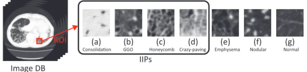
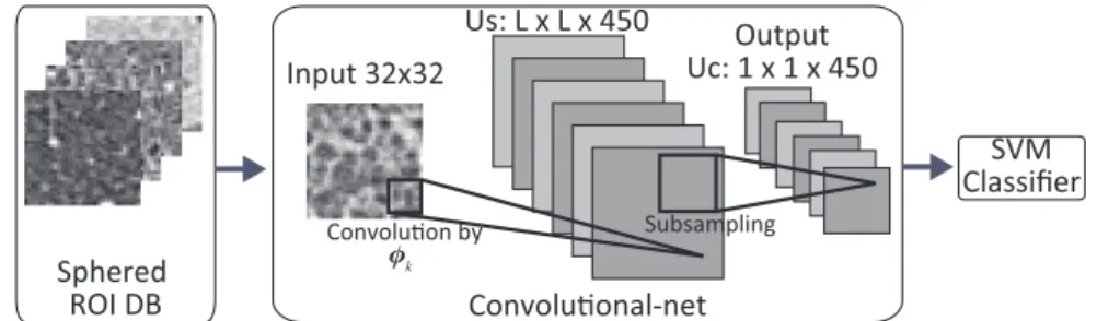
(2) Vol.2011-MPS-84 No.2 2011/7/18 IPSJ SIG Technical Report. Us: L x L x 450. For IIPs classification, several approach are proposed, and, in recent years, a “texton” base system are focused in classification of lung diseases6) . A texton means the clustered features from the collection of small patch of images, and texton base system use the collection of similarities between an input and each texton as a feature vector. Thus, our approach can be regarded as an extension of this texton base approach. In this study, we developed a prototype CAD system for classifying IIPs. Our CAD system take a segmented image which is taken from the HRCT image of lungs, and classify the input image into following named classes, that is, consolidation, ground-grass opacity (GGO), honeycomb, crazy-paving, nodular, emphysema and normal classes. The lesion of this disease is spread in lung, and has a lot of image patterns even in the same class. Fig.1 shows a typical image example of each disease HRCT image. The left shows an overview of the axial HRCT images of lungs including lesion, and the right shows segmented images of typical examples of lesion from the left image collections. The consolidation and GGO patterns are often appeared with the cryptogenic organizing pneumonia diseases (COPD). The GGO pattern is also often appeared in the non-specific interstitial pneumonia (NSIP). The crazy-paving pattern have reticular pattern with partial GGO patterns, which appeared in also NSIP. The honeycomb pattern has more rough mesh structure rather than that of the crazy-paving, and it appeared in idiopathic pulmonary fibrosis (IPF) or usual interstitial pneumonia (UIP).. Input 32x32. Output Uc: 1 x 1 x 450 SVM Classiﬁer. Sphered ROI DB Fig. 2. Convolu on by φk. Subsampling. Convolu onal-net. Schematic diagram of our CAD system using convolutional-net. In the convolutional-net part, each rectangle shows cell plane which includes same type of cells arranged in the 2D array.. sampling”1)3) . These calculation manners are originally proposed by Hubel & Wiesel7) . We treat each type of cell as arranged in 2-dimensional lattice called “cell plane”. The cell in a cell plane has same preferred vector except the receptive field position, which is just differ as the position of the cell in the cell plane. Introducing the cell plane structure, we can treat the connection between the cell planes as the convolution. Thus, we call this type of network as “convolutional-net”. In the center part of the Fig.2 shows a schematic diagram of the convolutional-net. Each rectangle in the part shows cell plane that includes same type of cells, and whole cells have only local connections. As in mathematical form, we denote the response of the S-cell at the location x in the k-th cell plane as us (x, k), and [ denote∑it as a convolution form: ] φ (ν)I(x + ν) k √∑ us (x, k) = ϕ √∑ ν − θk , (1) 2 2 ν φk (ν) ν I(x + ν) where ϕ[·] means the half-wave rectified { function: s if s > 0 , (2) ϕ[s] = 0 else θk means threshold value for the cell in the k-th cell plane, and φk (ν) means the connection weight for the relative location to x. Introducing a vector notation for index of receptive field ν, that is φk as φk (ν), I x [as I(x + ν), we can ] denote eq.(1) as: φk · I x us (x, k) = ϕ −θ (3) kφk k kI x k where dot operator in the numerator means the inner product of vectors, so that the first term in the function ϕ[·] means the similarity in the meaning of direction cosine. Thus, we can interpret the eq.(1) as two step calculation, that is the first step is calculation. 2. Method In this section, we explain about more detailed convolutional-net formulation and learning method of sparse coding using in our CAD system. 2.1 Structure of Convolutional- net The convolutional-net mainly consists of two types of cells. One is called “S-cell” which is used for feature extractor. The S-cell have local connection window called receptive field, and the local connection weight dictate preference of the S-cell, so that the local connection weight is sometimes called preferred vector. When an input is appeared to the receptive field, the S-cell calculates a similarity between the input and the preferred vector for responding. The other type of cell is called “C-cell” which is used for reduction of local input pattern deformation, such that shift, rotation, and so on. The C-cell calculates spatial pooling of the S-cell that have same preferred vector in the local area. This spatial pooling calculation is sometimes called “blurring” or “sub-. 2. c 2011 Information Processing Society of Japan.

(3) Vol.2011-MPS-84 No.2 2011/7/18 IPSJ SIG Technical Report. expressed by a linear combination of the feature ∑ p extraction vector {φk }: Ip ∼ ak φk .. of similarity between local input I x and the preferred vector φk , and the second is modulate the similarity by the threshold and half-wave rectification. The C-cell function also denote as a convolution for the spatial pooling in the S-cell plane:   ∑ uc (x, k) = ψ  ρ(ξ)us (x + ξ, k) , (4). (6). k. And the other point is the almost all the coefficients apk should be zero, that is only few feature extraction vectors support the image patch I p , and we call under this condition as “sparse” state. Then, we can introduce an objective as following: ∑ function ∑forpthe sparse coding p p p 2 J[{φk }, {ak }] = kI − ak φk k + λS({ak }), (7) p k ∑ log(1 + (apk )2 ). (8) S({apk }) =. ξ. where ξ indicates the connection location relative to the x, ρ(ξ) means the connection weight, and ψ[·] means the modulation function. In this study, to keep the network structure simple, we adopt following conditions. We assume connection between uc (x, k) have whole spatial pooling for us (x, k) which means uc (x, k) denote as a single unit uc (k) and it have full connection to the whole units in the previous plane us (x, k). Moreover, we also assume whole connection weight as homogeneous, that is ρ(ξ) = 1, and modulation function ψ[·] as linear modulation function ψ[u] = u. Hence, we can denote the C-cell for the k-th feature described ∑ in eq.(4) as: uc (k) = us (ξ, k). (5). p,k. In the eq.(7), the first term means a data fitting term and the second means a constraint for sparseness, and the parameter λ controls the balance between these two terms. Minimizing the objective function for the {φk } and {apk }, we can obtain the feature extracting vector set {φk } in the eq.(1). 3. Experiment. ξ. 3.1 Materials In order to evaluate our CAD system, we prepare 360 images, in which the number of each class are following: Consolidation:38, GGO:76, Honeycomb:49, Crazy-paving:37, Emphysema:54, Nodular:48, and Normal:58 cases. In usual, the HRCT image consists of 512 × 512 pixels. However, the whole image includes not only interest anatomy lung, but also another anatomies. Hence, in our system, we assume an input image is a part of HRCT image called “region of interest (ROI)” , which is segmented by a diagnostician. The size of ROI is configured as 32 × 32 pixels. Each ROI is segmented under the direction of a physician, and diagnosed by 3 physicians. The acquisition parameters of those HRCT images are as follows: Toshiba “Aquilion 16” is used for imaging device, each slice image consists of 512 x 512 pixels, and pixel size corresponds to 0.546 ∼ 0.826 mm, slice thickness are 1 mm. The number of patients is 69 males and 42 females with age 66.3 ± 13.4. The number of normal donor is 4 males and 2 females with age 44.3±10.3. The origin of these image data is provided Tokushima University Hospital. On the consolidation image, we cannot recognize the vessels since lesion have too much high CT values such like water. GGO represents the light distributed lesion, and. Now, we can consider the output of the convolutional-net uc (k) for the input I(x) as a kind of the conversion from the input to a feature vector, so that we should classify the feature vector into the class category. In order to classify uc (k), we introduce a support vector machine (SVM), which is developed in the field of machine learning, for classification in the next stage8) . 2.2 Learning of Preferred Feature by Sparse Coding For applying a convolutional-net into the natural image understanding, Gabor filters is usually adopted in the feature extractor connection φk . The Gabor filter is suitable for extraction of line or edge segment in the image, and those feature components are considered important in the field of natural scene understanding3)1) . However, it is doubtful that line or edge components in the segmented image of the IIPs is effective to the classification. Thus, we introduce learning base algorithm called sparse coding to determine the feature extraction vector set {φk }. The sparse coding is proposed by Olshausen & Field to explain the property of the simple cell in the brain9) . Denoting part of input image patch pattern set as {I p }, which have same size to the feature extraction vector φk , for training the feature extraction vectors where p is the pattern index. The idea of the sparse coding stands on the following points. One is the image patch I p should be. 3. c 2011 Information Processing Society of Japan.

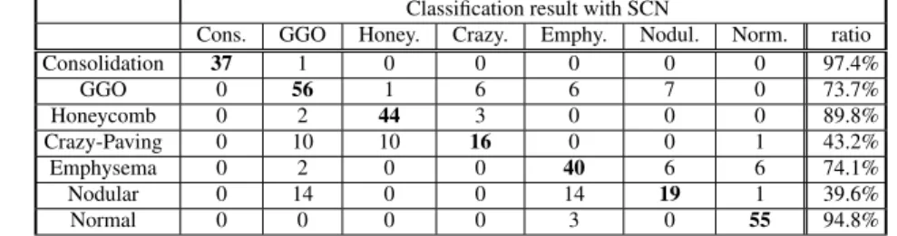
(4) Vol.2011-MPS-84 No.2 2011/7/18 IPSJ SIG Technical Report Classification ability by SCN with 20 × 20 feature extraction: Total correct ratio is 78.6% Classification result with SCN Cons. GGO Honey. Crazy. Emphy. Nodul. Norm. ratio Consolidation 36 2 0 0 0 0 0 94.7% GGO 0 59 2 2 0 13 0 77.6% Honeycomb 0 3 44 2 0 0 0 89.8% Crazy-Paving 0 3 0 28 1 5 0 75.7% Emphysema 0 3 0 0 44 7 0 81.5% Nodular 0 9 0 0 20 15 4 31.3% Normal 0 0 0 0 1 0 57 98.3%. Classification ability by GCN method with feature vector size 12 × 12: Total correct ratio is 58.1% Classification result with GCN Cons. GGO Honey. Crazy. Emphy. Nodul. Norm. ratio Consolidation 36 2 0 0 0 0 0 94.7% GGO 0 57 5 3 6 1 4 75.0% Honeycomb 1 5 36 3 1 3 0 73.5% Crazy-Paving 1 13 7 16 0 0 0 43.2% Emphysema 0 22 2 0 12 4 14 22.2% Nodular 0 13 6 4 11 10 4 20.8% Normal 0 4 0 0 10 2 42 72.4%. Table 1. Table 2. Classification ability by SCN method with feature vector size 12 × 12: Total correct ratio is 74.2% Classification result with SCN Cons. GGO Honey. Crazy. Emphy. Nodul. Norm. ratio Consolidation 37 1 0 0 0 0 0 97.4% GGO 0 56 1 6 6 7 0 73.7% Honeycomb 0 2 44 3 0 0 0 89.8% Crazy-Paving 0 10 10 16 0 0 1 43.2% Emphysema 0 2 0 0 40 6 6 74.1% Nodular 0 14 0 0 14 19 1 39.6% Normal 0 0 0 0 3 0 55 94.8%. Table 3. we can recognize vessels in contrast. Honeycomb appears geometrical patterns caused by the partial destruction of alveoli. Crazy-paving represents mixture state GGO and honeycomb. These 4 cases are IIPs class. Emphysema represents distributed low CT values area caused by the destruction of alveoli. Nodular represents small (< 5mm) nodule patterns. These 2 cases are not IIPs class, but another lung disease class. Normal class represents images collection from healthy donor. 3.2 Pre-processing for Input Before carrying out the sparse coding, we adopt “sphering”, which is sometimes called pre-whitening, by principal component analysis (PCA). The purpose of the sphering is to normalize the signal represented by each pixel, and to eliminate the effect of cross correlation to other pixels. When we denote the {Y p } as the data set of raw pixel data of ROIs, the sphering process can be denoted as following:. Λ= YYT p, (9). We fixed the number of feature vectors {φk } as 450 to satisfy overcomplete condition, and evaluated the effect of the vector length as {12 × 12, 16 × 16, 20 × 20}. The balance parameter λ in eq.(7) is set as 1.0 that is decided experimentally. For Minimization of the cost function (7), we apply a method proposed by Olshausen & Field, that is a kind of gradient decent along the parameters {apk } and {φk } alternately5) . Following equations are update rules: ∂J φknew ← φk + η (11) ∂φk ∂J (12) apk new ← apk + η p ∂ak where η is learning rate, that is fixed 0.0001 in this study. Eqs.(11) and (12) are applied alternately in the simulation. After training the feature extract vector set {φk }, we can apply convolutional-net calculation shown in eqs.(3) and (5) where threshold parameter θk = 0.0 for any k. As the result of convolutional-net calculation, we obtain a vector description, whose. I p = Λ− 2 Y p , (10) − 12 where h·ip means the average over patterns indexed by p, and Λ can be obtained by eigenvalue decomposing using PCA. As the result of sphering, the cross-correlation. matrix of pre-processed input, which denote as II T p , becomes a unit matrix, that is any pair of I p have no cross correlation. 3.3 Evaluation method In order to evaluate the ability of our CAD system, we apply leave one out crossvalidation (LOOCV) method10)11) . Applying this method, we left an input pattern for evaluation, and use another patterns to train the CAD system. Alternating the evaluation pattern, we evaluate the CAD system classification result on each occasion. 1. 4. c 2011 Information Processing Society of Japan.

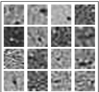
(5) Vol.2011-MPS-84 No.2 2011/7/18 IPSJ SIG Technical Report. element is composed by uc (k), for each pattern I p . Hence, we classify the vector to the IIPs’ category, and we use the SVM as the classifier that is provided by OpenCV with default parameters12) . Moreover, in order to compare the ability of our CAD with the conventional convolutional-net, we prepare Gabor function based system, that is {φk } as Gabor based system.In the following, we abbreviate sparse coding convolutional-net as SCN, and Gabor filter base convolutional-net as GCN.. best result in our evaluation. Each row shows the input class, and each column shows the classification class. Thus diagonal line shown in bold numbers represents the number of correct classifications. For example, in the consolidation patterns, 37 cases are classified as consolidation correctly, 1 case is classified as GGO. The total correct ratio is shown in the last column. From the Table 1, we can see the correction ratio of all the classes except nodular class are over 75%. Especially, seeing the normal class column of the Table 1, a type II error called false negative, that is the failure probability of finding diseases, is nothing except nodular class. The nodular class is not category of IIPs, and its HRCT image does not have specific texture feature, but have only local sphere like patterns. Hence, the whitening pre-process, which is for normalization and elimination of cross correlation, may reduce this local feature, so that whitening may makes low classification ratio as the result. Anyway, improving of nodular class performance is a future work. Table2 shows the result of classification performance by the GCN which is a modified model proposed by Kuwahara et al.13) . Kuwahara et al. have applied Gabor filter for feature extraction, and AdaBoost for classification. We substitute this AdaBoost part for a SVM in order to compare with SCN. The scale of feature extractor φk is 12 × 12 that is the best one in the examined Gabor feature scales. Table 3 shows the GCN result of the same feature extractor scale. Comparing the Table 2 with the Table3, we can see the classification performance of the GCN have similar tendency to the SCN, however, total performance of the SCN is clearly improved from the GCN. Especially, we can see the performance for the emphysema and the crazy-paving classes are dominantly improved. Roughly speaking, the crazy-paving class is a intermediate image between GGO and Honeycomb, and we can estimate that Gabor based filters, which is used in the GCN for line or edge component extraction, are not sufficient for feature extraction. Comparing Tables 1 and 2, which are different scale of φk , the performance of the large size φk is improved for the crazy-paving class. This result comes from the reducing of the miss classification to the honeycomb class, so that we can estimate large size φk is suitable for the extracting honeycomb structure.. 4. Results Figure 3 shows the several examples of feature extract vectors of φk . Since the HRCT ROI images are not sort of natural images, the obtained bases φk are not similar to the Gabor filters that can be obtained by the sparse coding with natural scene processing5) . This difference makes classification performance as following. Table 1 shows the detail classification result by a confusion matrix. The Table 1 is a result of a SCN in which the length of feature vector φk is 20 × 20 network. This is the. 5. Conclusion. Fig. 3. In this study, we evaluated the sparse coding base convolutional-net for the multi-class IIP classification. Comparing the correction performance with the simple GCN that is a. Several examples of feature extract vector φk obtained by sparse coding.. 5. c 2011 Information Processing Society of Japan.

(6) Vol.2011-MPS-84 No.2 2011/7/18 IPSJ SIG Technical Report. modified of the previous model, we can obtain an improvement result. Especially, type II error frequency of GCN is larger than that of the SCN. From the clinical point of view, we can conclude the several training method for the feature-extracting vector set {φk } is effective. Gangeh et al. also pointed out the similar tendency in their “texton” based model6) . We consider the total performance of the classification rate is not so much bad, however, we should improve the performance of our SCN for the practical CAD system. In the future works, in order to improve our SCN performance, we should find a tuning method or principle. In this work, we show the preliminary result for the feature extractor size effect. We can estimate the larger one is suitable for finding the structure such like crazy-paving and honeycomb, so that we should find optimal size of the feature extractor φk . One solution is that multi-scale feature extractor such like Lowe model may be effective for this problem14) .. Texton-Based Approach for the Classification of Lung Parenchyma in CT Images, MICCAI, LNCS 6363, No.3, Springer-Verlag Berlin Heidelberg, pp.595–602 (2010). 7) Hubel, D.H. and Wiesel, T.N.: Receptive fields and functional architecture of monkey striate cortex, J. Physiol., Vol.195, No.1, pp.215–243 (1968). 8) Shölkopf, B., Sung, K.-K., Burges, C., Girosi, F., Niyogi, P., Poggio, T. and Vapnik, V.: Comparing Suport Vector Machines with Gaussian Kernels to Radial Basis Function Classifiers, IEEE Trans. on Signal Processing, Vol.45, No.11, pp.2758–2765 (1997). 9) Olshausen, B. A. and Field, D. J.: Emergence of simple-cell receptive field properties by learning a sparse code for natural images., Nature, Vol.381, pp.607–609 (online), DOI:doi:10.1038/381607a0 (1996). 10) Stone, M.: Cross-validation: A review., Math.Operations.Stat.Ser.Stat, Vol.9, No.1, pp.127– 139 (1978). 11) Bishop, C.M.: Pattern Recogition and Machine Learning, Springer (2006). 12) Bradski, G.: The OpenCV Library, Dr. Dobb’s Journal of Software Tools (2000). 13) Kuwahara, M., Kido, S. and Shouno, H.: Classification of patterns for diffuse lung diseases in thoracic CT images by AdaBoost algorithm, Proceedings of SPIE, Vol. 7260, (online), DOI:http://dx.doi.org/10.1117/12.811497 (2009). 14) Mutch, J. and Lowe, D.: Object class recognition and localization using sparse features with limited receptive fields, International Journal of Computer Vision, Vol.80, No.1, pp.45–57 (online), DOI:DOI:10.1007/s11263-007-0118-0 (2008).. Acknowledgement We thank Professor Junji Ueno, Tokushima University. He provided us several advices for this study as well as a set of high resolution CT image of IIPs. This work is supported by Grant-in-Aids for Scientific Research (C) 21500214, and Innovative Areas 21103008, MEXT, Japan. References 1) Fukushima, K.: Neocognitron: A Self-Organizing Neural Network Model for a Mechanism of Pattern Recognition Unaffected by Shift in Position, Biological Cybernetics, Vol.36, No.4, pp.193–202 (1980). 2) Shouno, H.: Recent Studies around the Neocognitron, Neural Information Processing, 14th International Conference, ICONIP 2007, Kitakyushu, Japan, November 13-16, 2007, Revised Selected Papers, Part I (Ishikawa, M., Doya, K., Miyamoto, H. and Yamakawa, T., eds.), Lecture Notes in Computer Science, Vol.4984, Springer, pp.1061–1070 (2007). 3) Huang, F.J. and LeCun, Y.: Large-scale Learning with SVM and Convolutional Netw for Generic Object Recognition., 2006 IEEE Computer Society Conference on Computer Vision and Pattern Recognition, IEEE Computer Society CVPR’06 (2006). 4) Riesenhuber, M. and Poggio, T.: Hierachical modesl of object recognition in cortex, Nature Neuroscience, Vol.2, pp.1019–1025 (1999). 5) Olshausen, B.A. and Field, D.J.: Sparse coding with an overcomplete basis set: A strategy employed by V1?, Vision Research, Vol.37, No.23, pp.3311–3325 (online), DOI:doi:10.1016/S0042-6989(97)00169-7 (1997). 6) Gangeh, M.J., Sorensen, L., Shaker, S.B., Kamel, M.S., de Bruijne, M. and Loog, M.: A. 6. c 2011 Information Processing Society of Japan.

(7)