Sparse Estimation of Spike-Triggered Average

全文

(1)Vol.2013-MPS-93 No.4 2013/5/23. IPSJ SIG Technical Report. Sparse Estimation of Spike-Triggered Average Shimpei Yotsukura1. Toshiaki Omori2. Kenji Nagata1. Masato Okada1,3. Abstract: The spike-triggered average (STA) and phase response curve characterize the response properties of sin-. gle neurons. A recent theoretical study proposed a method to estimate the phase response curve by means of linear regression with Fourier basis functions. In this study, we propose a method to estimate the STA by means of sparse linear regression with Fourier and polynomial basis functions. In the proposed method, we use sparse estimation with L1 regularization to extract substantial basis functions for the STA. We show using simulated data that the proposed method achieves more accurate estimation of the STA than the simple trial average used in conventional method. Keywords: spike-triggered average, linear regression, L1 regularization, model selection, curve fitting. 1. Introduction Neurons are encoders that transform time series of inputs into spikes. Spike-triggered analysis has been used extensively to estimate the statistical properties of the time-varying inputs inducing the spikes [1], [2], [3], [4], [5]. In particular, the spike-triggered average (STA), first-order statistics of the spike-triggered analysis, corresponds to an average of time series of inputs that induce the spikes. The STA has been used in physiological experiments to estimate receptive fields in neural systems [6], [7], [8]. To obtain the STA from experimental results, we need to observe a spike train from a specific neuron and calculate an average of time series of inputs that induce the spike train. In previous studies, the STA has been calculated simply as a trial average of inputs inducing a finite number of spikes [9]. However, the number of observable spikes from a specific neuron is limited in physiological experiments. Due to this limitation, the STA calculated as the simple trial average is rather noisy, which makes it difficult to obtain the true STA accurately. A recent study proposed a method to estimate phase response curve (PRC) by using linear regression with Fourier basis functions [10]. The PRC is a periodic function that characterizes the response properties of single neurons. This method has been shown to accurately estimate the PRC from experimental data. Since the STA is known to be proportional to a derivative of the PRC [9], it would seem that the linear regression would be effective for estimating the STA as well as the PRC. However, the STA would be a discontinuous function whereas the PRC is a periodic continuous function. This would make it difficult to estimate the STA using linear regression with only Fourier basis functions, and it is unclear what kinds of basis functions are appropriate to 1. 2. 3. Graduate School of Frontier Sciences, The University of Tokyo, 5-1-5, Kashiwanoha, Kashiwa, 277-8561, Japan Graduate School of Engineering, Kobe University, 1-1, Rokkodai, Nadaku, Kobe, 657-8501, Japan Brain Science Institute, RIKEN, 2-1, Hirosawa, Wako, Saitama, 3510198, Japan. c 2013 Information Processing Society of Japan ⃝. estimate the STA by linear regression. In this paper, we propose an algorithm to estimate the STA based on sparse estimation by using L1 regularization [11], [12], [13], [14]. In the proposed method, essential basis functions for the STA are extracted automatically by means of sparse linear regression using the L1 regularization. Appropriate basis functions for estimating the STA are evaluated by applying the proposed method to simulated data obtained using the Morris-Lecar model [15]. We show using the simulated data that the proposed method can estimate the STA more accurately than the conventional method using the simple trial average.. 2. Spike-Triggered Average In this study, we propose an algorithm to estimate the suprathreshold STA [9], [16]. Hereafter, we call the suprathreshold STA simply the STA. Let V (t) be a membrane potential of a neuron at time t. The neuron is assumed to emit a spike when the membrane potential V (t) exceeds a firing threshold Vth . We assume that the neuron receives an input current I (t) as I (t) = I0 + ξ (t) ,. (1). where I0 is a constant current and ξ (t) is a noise current obeying the white Gaussian noise with the average 0 and the variance σ2 . The constant current I0 is assumed to be sufficiently large to generate spikes without noise input ξ (t). As shown in Fig. 1, we assume that the neuron generates spikes at time tk (k = 1, 2, · · · , K) by the constant and noise currents. The STA, C0 (τ), is defined as C0 (τ) = lim. K→∞. K 1 ∑ ξ (tk − τ) , K k=1. (2). where K indicates the number of spikes. ξ (tk − τ) represents the noise current that comes τ before the k-th spike. Namely, the STA is an average of the noise current ξ (tk − τ) preceding spikes. Although the definition of the STA, C0 (τ), assumes an infinite number of spikes, we cannot obtain an infinite number of spikes in physiological experiments. The STA is therefore calculated ap1.

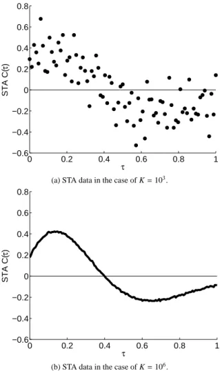
(2) Vol.2013-MPS-93 No.4 2013/5/23. IPSJ SIG Technical Report. 0.8 0.6 0.4 STA C(τ). I(t) I0. τ. t1. t3. t2. t. 0 −0.2. τ. −0.4. ξ(t1-τ). −0.6 0. ξ(t2-τ). 0.2. 0.4. τ. 0.6. 0.8. 1. 0.8. 1. (a) STA data in the case of K = 103 .. ξ(t3-τ). 0.8. τ average STA C0(τ). 0.6. A schematic diagram of the spike-triggered average (STA). A neuron is assumed to receive the input current I (t) consisting of the constant current I0 and the noise current ξ (t) and generate spikes at time {tk }. The STA is defined as the average of the noise current ξ (tk − τ) preceding the spike time tk by the interval τ.. proximately with a finite number of spikes K obtained from experimental and numerical data. We show an example of the STA calculated as the trial average with the finite number of spikes in Fig. 2(a). We found that the STA calculated as the trial average is noisy, and thus it is difficult to calculate the STA accurately using the conventional method based on the trial average. Hereafter, we call the STA calculated by the trial average with the finite number of spikes simply the STA data.. 3. Proposed Method. STA C(τ). 0.4. τ Fig. 1. 0.2. 0.2 0 −0.2 −0.4 −0.6 0. 0.2. 0.4. τ. 0.6. (b) STA data in the case of K = 106 . Fig. 2. Examples of STA data obtained by the type I Morris-Lecar model. (a) STA data in the case in which the number of spikes, K, is 103 . The STA data is noisy if the number of spikes, K, is small. (b) STA data in the case in which the number of spikes, K, is 106 . The STA data converges to the true STA if the number of spikes, K, is sufficiently large. The true STA can be a discontinuous periodic function since C0 (0) is not equal to C0 (T ), as shown in (b). Here the firing period T is set to be 1.. In this section, we propose an algorithm to estimate the STA with linear regression based on L1 regularization in order to accurately estimate the true STA from noisy STA data. 3.1 Sparse Estimation of the STA based on L1 Regularization We consider a situation in which we obtain the STA data with N points {(τ1 , C (τ1 )) , · · · , (τN , C (τN ))} by physiological experiments. Each value of the STA data, C (τi ), is assumed to consist of the true STA, C0 (τi ), and noise. In this study, we propose an algorithm to estimate the true STA, C0 (τ), from the STA data by using linear regression with basis functions. The true STA, C0 (τ), is assumed to } be expressed by a linear { combination of basis functions f j (τ) , as C0 (τ) = a1 f1 (τ) + · · · + a M f M (τ) =. M ∑. a j f j (τ) ,. (3). j=1. where M is the number of basis functions and {a1 , · · · , a M } are real coefficients. We consider a linear regression problem to. c 2013 Information Processing Society of Japan ⃝. determine the coefficients {a1 , · · · , a M } based on the STA data {(τ1 , C (τ1 )) , · · · , (τN , C (τN ))} in order to obtain the regression model of the STA. If we use an excessive number of basis functions in the linear regression, we run the risk of overfitting, which would result in a failed estimation of the true STA since the regression model is strongly influenced by the noise in such cases. Thus, we need to extract only essential basis functions to estimate the STA accurately. In this study, we introduce L1 regularization [11], [12], [13], [14] in order to extract essential basis functions automatically based on the STA data. The L1 regularization is defined to determine the coefficients {a1 , · · · , a M } so as to minimize the following objective function: 2.

(3) Vol.2013-MPS-93 No.4 2013/5/23. IPSJ SIG Technical Report. E (a1 , · · · , a M ) =. N ∑. (C (τi ) − C0 (τi ))2 +. M ∑. i=1.

(4)

(5) λ j

(6)

(7) a j

(8)

(9). j=1.  2 N  M ∑ ∑    = a j f j (τi ) C (τi ) − i=1. +. j=1. M ∑.

(10)

(11) λ j

(12)

(13) a j

(14)

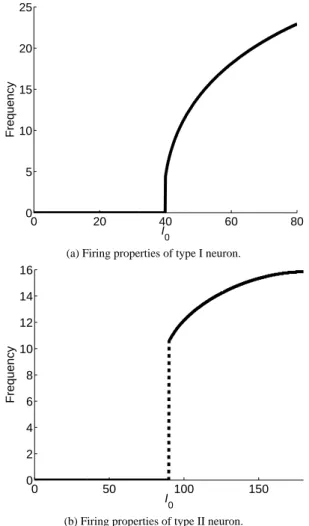
(15) .. (4). j=1. Here, λ j are assumed to be positive constants. The first term of the objective function E represents a discrepancy between the regression model and the STA data. The second term is a penalty term that prevents absolute values of coefficients from increas{ } ing. By this penalty term, the coefficients a j for redundant basis functions are likely to be exactly zero. Thus, essential basis functions can be extracted using the L1 regularization, and the model selection can be realized automatically. This kind of estimation using Eq. (4) is called sparse estimation. 3.2 Design of basis functions and regularization weights The accuracy of the regression in Eq. (3) is determined by what kinds of functions we prepare for redundant basis functions { f1 (τ), · · · , f M (τ)}. Fourier basis functions were used in the linear regression of the phase response curve (PRC) in a previous study by Galán et al. [10]. The PRC describes a phase shift induced by perturbation given to a periodically firing neuron and characterizes the response properties of single neurons. Since the PRC is a periodic function, the previous study [10] used the Fourier basis functions. Ermentrout et al. analytically showed that the STA is proportional to a derivative of the PRC [9]. Therefore, we consider a regression of the STA using the Fourier basis functions as well as the PRC. Since a derivative of a continuous function is not always continuous, the STA, which is proportional to a derivative of the PRC, can be discontinuous. Actually, as shown in Fig. 2(b), the STA can be discontinuous since C0 (0) is not equal to C0 (T ). If we perform a regression of the STA using only Fourier basis functions, it is expected that high-frequency components of the Fourier basis functions are needed to express the discontinuity of the STA, even when the true STA may not include the highfrequency components. In this study, we used the Fourier basis functions and polynomial basis functions in order to express the discontinuity of the STA, as C0 (τ) =a1 +. Df ∑. a(k+1) cos (2kπτ). k=1. +. Df ∑. a(k+D f +1) sin (2kπτ). k=1. +. Dp ∑. a(k+2D f +1) τk ,. (5). sparse regression using a sufficiently large number of the Fourier and polynomial basis functions by setting the maximum order of each kind of basis functions D f and D p to be sufficiently large. The sparse estimation is conducted using the L1 regularization to extract only essential basis functions for the STA. The regularization weights λ j in Eq. (4) should be determined in order to perform the L1 regularization. Absolute values of the coefficients for high-frequency components of the Fourier basis functions are expected to be relatively small in the true STA. On the other hand, noise contains large high-frequency components. In this study, we propose a method that strongly penalizes extraction of high-frequency components of Fourier basis functions. For this purpose, we set the regularization weights λ j as    ( j − 1) λ   )   ( λj =  j − Df − 1 λ      λ. ( ) if 2 ≤ j ≤ D f + 1 ( ) if D f + 2 ≤ j ≤ 2D f + 1 (otherwise) ,. (6). where λ is a positive constant. In Eq. (6), the regularization weights are set to be proportional to the frequency of the Fourier basis functions. Namely, the regularization weight λ j for k-th order Fourier basis functions cos(2πkτ) and sin(2πkτ) is set to be λ j = kλ. The constant λ is determined so as to minimize a generalization error calculated by a cross-validation method.. 4. Results In this section, we apply the proposed algorithm to STA data obtained by simulation using a neuron model. 4.1 Morris-Lecar Model In this study, we used the Morris-Lecar model as a neuron model [15], [17]. In this model, the dynamics of the membrane potential V (t) obey the following differential equation: C. dV (t) = − g¯ Ca m∞ (V (t)) (V (t) − VCa ) dt − g¯ K w (t) (V (t) − VK ) − g¯ L (V (t) − VL ) + I (t) .. (7). Here, Eq. (7) describes the relationship between ion currents and the membrane potential. We describe further details of the Morris-Lecar model in the Appendix. Neurons are classified into type I and II neurons according to their firing properties [16], [17], [18]. The Morris-Lecar model can mimic both types by using appropriate parameter settings. We show the difference in firing properties between the two in Fig. 3. For both type I and II neurons, a neuron fires periodically if it receives a sufficiently large constant current I0 . Firing frequency of the type I neuron is continuous, as shown in Fig. 3(a), whereas that of the type II neuron changes discontinuously, as shown in Fig. 3(b). We apply the proposed method to the STA data of both type I and II obtained by the Morris-Lecar model.. k=1. where the firing period T is set to be 1. D f and D p are the maximum order of the Fourier and polynomial basis functions, respectively. Here, it is unclear which order of the Fourier and polynomial basis functions are needed in advance. We perform. c 2013 Information Processing Society of Japan ⃝. 4.2 Settings of Numerical Simulations and Sparse Estimation The STA data is numerically obtained by the Morris-Lecar model with the constant and noise currents I(t) = I0 + ξ(t). The 3.

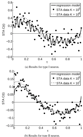
(16) Vol.2013-MPS-93 No.4 2013/5/23. IPSJ SIG Technical Report. 25. 0.8. regression model STA data K = 103. 0.6. 20. STA data K = 106 STA C(τ). Frequency. 0.4 15. 10. 0.2 0 −0.2. 5. −0.4 0 0. 20. 40 I. 60. 80. −0.6 0. 0. 0.2. 0.4. (a) Firing properties of type I neuron.. 14 12. 0.15. 1. regression model STA data K = 105. 0.1. 8 6 4. 0.05 0 −0.05. 2 50. I0. 100. −0.1. 150. −0.15 0. (b) Firing properties of type II neuron. Fig. 3. 0.8. STA data K = 107. 10. 0 0. 0.6. (a) Results for type I neuron.. 0.2. STA C(τ). Frequency. 16. τ. Firing properties of neurons. Firing frequency of type I neuron is continuous whereas that of type II neuron is discontinuous.. 4.3 Results of the Proposed Method In this section, we show the results of the proposed method. Namely, we perform sparse estimation with the regularization weights λ j obeying Eq. (6). The solid line in Fig. 4(a) shows the regression model estimated by the proposed method. Here, the proposed method is applied to the STA data calculated using the number of spikes K = 103 . We find that the discontinuity C(0) , C(T ) is expressed in the regression model estimated by the proposed method. From Table 1(a), we also find that one polynomial basis function is extracted in addition to Fourier basis functions. Furthermore, the low-frequency components of the. c 2013 Information Processing Society of Japan ⃝. 0.4. τ. 0.6. 0.8. 1. (b) Results for type II neuron. Fig. 4. constant current I0 is assumed to be sufficiently large to generate spikes periodically without noise input. We apply the sparse estimation algorithm to the STA data. In this section, the estimation of the STA is performed in two ways. The first case is the proposed method, in which the regularization weights λ j are assumed as in Eq. (6). In the second case, the regularization weights λ j are set to be constant λ. The value of λ is determined by using 10-fold cross-validation. We use the STA data calculated using the number of spikes 102 , 103 , 104 , and 105 in type I neuron and the STA data calculated using the number of spikes 103 , 104 , 105 , and 106 in type II neuron. The maximum order of the Fourier basis functions, D f , is set to be 25 and that of the polynomial, D p , is 50.. 0.2. Results of the proposed method applied to noisy STA data that were obtained using the Morris-Lecar model. (a) Results for type I neuron. (b) Results for type II neuron. Dots represent the noisy STA data calculated by using the small number of spikes (K = 103 for type I neuron and K = 105 for type II neuron). The solid line shows a regression model of the STA estimated from the noisy STA data by using the proposed method while the dashed line shows less noisy STA data calculated by using a sufficiently large number of spikes (K = 106 for type I neuron and K = 107 for type II neuron).. Table 1 The number of the basis functions extracted by the proposed method, and the number of all basis functions. Top row shows the number of spikes K used to calculate the STA data. Middle row shows the number of both Fourier and polynomial basis functions. Bottom row shows the number of the polynomial functions only. (a) Results for type I neuron. K No .extracted / All (polynomial). 102 3/101 1/50. 103 7/101 1/50. 104 9/101 4/50. 105 25/101 3/50. (b) Results for type II neuron. K No. extracted / All (polynomial). 103 0/101 0/50. 104 3/101 1/50. 105 6/101 1/50. 106 9/101 2/50. Fourier basis functions are extracted by strongly penalizing highfrequency components. As discussed above, we see that essential basis functions of the STA are extracted and the model selection is accurately realized by the proposed sparse estimation. Figure 4(b) and Table 1(b) show estimated results for type II neuron. We find that essential basis functions of the STA are extracted in the 4.

(17) Vol.2013-MPS-93 No.4 2013/5/23. IPSJ SIG Technical Report. 0. 0.8. 10. proposed method conventional method. regression model STA data K = 103. 0.6. STA C(τ). Generalization error. STA data K = 106 0.4 −1. 10. 0.2 0 −0.2 −0.4. −2. 10. 2. 10. 3. 4. 10. 10. −0.6 0. 5. 10. K. τ. 0.6. 0.2. 0. proposed method conventional method. 0.8. 1. regression model STA data K = 105. 0.15. STA data K = 107 0.1 STA C(τ). Generalization error. 0.4. (a) Results for type I neuron.. (a) The generalization error in type I neuron.. 10. 0.2. −1. 10. 0.05 0 −0.05 −0.1. −2. 10. −0.15 0 3. 10. 4. 5. 10. 10. 0.2. 0.4. 6. 10. K (b) The generalization error in type II neuron. Fig. 5 Generalization error in the proposed method. The proposed method was applied to the STA data obtained by simulation using the MorrisLecar model. (a) The generalization error in type I neuron. (b) The generalization error in type II neuron. The horizontal axis represents the number of spikes, K, and the vertical axis represents the generalization error. Even when the number of spikes used in the proposed method was only ten percent of that used in the conventional method, the proposed method had a similar performance to the conventional method.. τ. 0.6. 0.8. 1. (b) Results for type II neuron. Fig. 6. Results of L1 regularization in the case when λ j = λ. (a) Results for type I neuron. (b) Results for type II neuron. Dots represent the noisy STA data calculated by using the small number of spikes. A solid line is the regression model of the STA estimated by L1 regularization from the noisy STA data. A dashed line represents the less noisy STA data calculated by using the sufficiently large number of spikes.. Table 2 The number of extracted basis functions in the case of λ j = λ, and the number of all basis functions. (a) Results for type I neuron. K No. extracted / All (polynomial). case of type II neuron as in the case of type I neuron. Next, we evaluate the discrepancy between the conventional method using the simple trial average and the proposed method. We evaluate the generalization error calculated by the root mean square error between the target STA data and the regression model. The target STA data corresponds to the STA data with the sufficiently large number of spikes. The number of spikes of the target STA data is set to be K = 106 for type I neuron and K = 107 for type II neuron. As shown in Fig. 5, the discrepancy of the proposed method using the STA data with the number of spikes K is similar to that of the conventional method using the STA data with the number of spikes 10K. From these results, we find that even when the number of spikes used in the proposed method is only ten percent of that used in the conventional method, the proposed method had a similar performance to the conventional method.. c 2013 Information Processing Society of Japan ⃝. 102 1/101 0/50. 103 16/101 0/50. 104 27/101 1/50. 105 44/101 5/50. (b) Results for type II neuron. K No. extracted / All (polynomial). 103 4/101 0/50. 104 19/101 1/50. 105 19/101 1/50. 106 47/101 1/50. 4.4 Case of Constant Regularization Weights In this section, we consider a case in which all the regularization weights λ j for both Fourier and polynomial basis functions are constant value λ, not dependent on j. We show the results of this case in Fig. 6 and Table 2. As shown in Fig. 6, the highfrequency components of the Fourier basis functions are extracted due to noise in the STA data, and the regression model is too wavy. The polynomial functions are difficult to extract, as shown in Table 2, since the discontinuity, C(0) , C(T ), is intended to be expressed by the high-frequency components of the Fourier basis functions, not the polynomial basis functions. Thus, we fail to 5.

(18) Vol.2013-MPS-93 No.4 2013/5/23. IPSJ SIG Technical Report. extract only low-frequency components and the regression model is strongly influenced by the noise. As discussed above, the proposed method is effective for estimating the true STA from the experimental STA data in the case of §4.3. On the other hand, it is difficult to extract important components in the case of §4.4.. Appendix. 5. Conclusion. The Morris-Lecar model is a system obeying the following equation:. lectively Driven by Differential Stimulus Features, Neural Comput., Vol. 20, No. 10, pp. 2418-2440 (2008).. A.1 Morris-Lecar Model. In this paper, we proposed an algorithm to estimate the STA using linear regression. We introduced sparse estimation using L1 regularization to estimate the STA and employed Fourier basis functions and polynomial basis functions in the linear regression. Using simulated data obtained by the Morris-Lecar model, we have shown that extraction of the basis functions with high generalization performance can be achieved by penalizing the extraction of high-frequency components of the Fourier basis functions. We have also shown that even when the number of spikes used in the proposed method is only ten percent of that used in the conventional method, the proposed method has a similar performance to the conventional method. References [1] [2] [3] [4] [5] [6] [7] [8] [9] [10] [11] [12] [13]. [14] [15] [16] [17] [18]. De Boer, E. and Kuyper, P.: Triggered Correlation, IEEE Transact. Biomed. Eng., Vol. 15, pp. 169-179 (1968). Bryant, H.L. and Segundo, J.P.: Spike Initiation by Transmembrane Current: A White-Noise Analysis., J. Physiol., Vol. 260, pp. 279-314 (1976). Chichilnisky, E.J.: A Simple White Noise Analysis of Neuronal Light Responses, Network: Comput. Neural Syst., Vol. 12, pp. 199-213 (2001). Dayan, P. and Abbott, L.F.: Theoretical Neuroscience: Computational and Mathematical Modeling of Neural Systems, MIT Press (2001). Simoncelli, E.P., Paninski, L., Pillow, J. and Schwartz, O.: Characterization of Neural Response with Stochastic Stimuli: The Cognitive Neurosciences (Gazzaniga, M., ed.), MIT Press (2004). Fries, P., Reynolds, J.H., Rorie, A.E. and Desimone, R.: Modulation of Oscillatory Neuronal Synchronization by Selective Visual Attention, Science, Vol. 291, No. 5508, pp. 1560-1563 (2001). Segev, R., Goodhouse, J., Puchalla, J. and Berry II, M.J.: Recording Spikes from a Large Fraction of the Ganglion Cells in a Retinal Patch, Nat. Neurosci., Vol. 7, pp. 1155-1162 (2004). Farrow, K., Haag, J. and Borst, A.: Nonlinear, Binocular Interactions Underlying Flow Field Selectivity of a Motion Sensitive Neuron, Nat. Neurosci., Vol. 9, pp. 1312-1320 (2006). Ermentrout, G.B., Galán, R.F. and Urban, N.N.: Relating Neural Dynamics to Neural Coding, Phys. Rev. Lett., Vol. 99, 248103 (2007). Galán, R.F., Ermentrout, G.B. and Urban, N.N.: Efficient Estimation of Phase-Resetting Curves in Real Neurons and its Significance for Neural-Network Modeling, Phys. Rev. Lett., Vol. 94, 158101 (2005). Tibshirani, R.: Regression Shrinkage and Selection via the Lasso, J. Royal. Statist. Soc. B, Vol. 58, No.1, pp. 267-288 (1996). Kabashima, Y., Wadayama, T., and Tanaka, T.: A Typical Reconstruction Limit for Compressed Sensing Based on L p -Norm Minimization, J. Stat. Mech., Vol. 2009, L09003 (2009). Mimura, K.: Compressed Sensing - Sparse Recovery and its Algorithms -, Theory and Scientific Applications in Time-Frequency Analysis, Research Institute for Mathematical Sciences, No.1803, pp. 26-56 (2012). (in Japanese). Tomioka, R. and Sugiyama, M.: Dual Augmented Lagrangian Method for Efficient Sparse Reconstruction, IEEE Signal Processing Letters, Vol. 16, No. 12, pp. 1067-1070 (2009). Morris, C. and Lecar, H.: Voltage Oscillations in the Barnacle Giant Muscle Fiber, Biophys. J., Vol.35, No.1, pp. 193-213 (1981). Omori, T., Aonishi, T. and Okada, M.: Switch of Encoding Characteristics in Single Neurons by Subthreshold and Suprathreshold Stimuli, Phys. Rev. E, Vol.81, 021901 (2010). Rinzel, J. and Ermentrout, G.B.: Analysis of Neural Excitability and Oscillations, Methods in Neuronal Modeling (Koch, C. and Segev, I. eds.), MIT Press (1998). Mato, G. and Samengo, I.: Type I and Type II Neuron Models are Se-. c 2013 Information Processing Society of Japan ⃝. C. dV (t) = −¯gCa m∞ (V (t)) (V (t) − VCa ) dt − g¯ K w (t) (V (t) − VK ) − g¯ L (V (t) − VL ) + I (t) ,. dw (t) w∞ (V (t)) − w (t) , =ϕ dt τw (V (t)) { ( )} V (t) − V1 m∞ (V (t)) = 0.5 1 + tanh , V2 { ( )} V (t) − V3 w∞ (V (t)) = 0.5 1 + tanh , V4 1 ( V(t)−V ) . τw (V (t)) = cosh 2V4 3. (A.1) (A.2) (A.3) (A.4) (A.5). The variable, V (t), represents the membrane potential of a neuron and w (t) is a gate variable of potassium. VCa , Vk and VL are the reversal potentials of calcium, potassium, and leak channel, respectively. g¯ Ca , g¯ K , and g¯ L represent the maximum value of channel conductance. C is a membrane capacitance. The parameters are set as shown in Table A·1.. type I type II type I type II. Table A·1 Parameters of the Morris-Lecar model. V1 V2 V3 V4 g¯ Ca g¯ K g¯ L -1.2 18 12 17.4 4.0 8.0 2 -1.2 18 2 30 4.4 8.0 2 VCa VK VL C ϕ Vth I0 σ 120 -84 -60 20 0.04 -13.3 41 5 120 -84 -60 20 1/15 -11.0 90 10. 6.

(19)