LAGRANGIAN RELAXATION AND PEGGING TEST FOR LINEAR ORDERING PROBLEMS
Noriyoshi Sukegawa Yoshitsugu Yamamoto Liyuan Zhang
University of Tsukuba
(Received June 9, 2011; Revised September 26, 2011)
Abstract We develop an algorithm for the linear ordering problem, which has a large number of ap-plications such as triangulation of input-output matrices, minimizing total weighted completion time in one-machine scheduling, and aggregation of individual preferences. The algorithm is based on the La-grangian relaxation of a binary integer linear programming formulation of the problem. Since the number of the constraints is proportional to the third power of the number of items and grows rapidly, we propose a modified subgradient method that temporarily ignores a large part of the constraints and gradually adds constraints whose Lagrangian multipliers are likely to be positive at an optimal multiplier vector. We also propose an improvement on the ordinary pegging test by using the problem structure.
Keywords: Combinatorial optimization, linear ordering problem, Lagrangian relax-ation, Lagrangian dual, subgradient method, pegging test
1. Introduction
The problem we consider in this paper is to find a linear ordering of n items when their pairwise comparison data are given. The data are given by an n×n matrix C := [cij]i,j=1,...,n
such that its (i, j)th element carries the amount of profit made when item i is ranked prior to item j. Choosing an appropriate matrix C lets the problem embrace the ranking aggregation problem, which is known as Kemeny’s problem, the minimum violations ranking problem, and Slater’s problem. See the survey paper by Charon and Hudry [8] and the book by Reinelt [25]. The problem is formulated as a linear integer programming problem. The polytope being the convex hull of binary vectors each corresponding to a linear ordering was named the linear ordering polytope and investigated by Gr¨otschel et al. [17]. They introduced some facet-defining valid inequalities of the polytope, and proposed a linear-programming-relaxation-based algorithm for the problem in [16]. For subsequent researches on the linear ordering polytope, see [4, 10, 20, 23]. Their approach was further extended by Mitchell and Borchers [21, 22], who proposed a cutting plane algorithm based on a primal-dual interior point method, and solved problems with as many as 250 items. Since the problem is NP -hard, see e.g., Section 2 of [8], there have been proposed several heuristic methods, e.g., Lagrangian heuristic method in [3], scatter search method in [5], linear ordering construction heuristics in [9], Goddard’s method in [14], variable neighborhood local search method in
[15]. Charon and Hudry [7] made an experiment of a branch-and-bound method with
Lagrangian relaxation and some heuristics.
The binary integer programming formulation of the linear ordering problem has an O(n3) of inequality constraints. This feature makes the problem hard to solve. We propose a Lagrangian relaxation algorithm that considers a small fraction of the inequality constrains, and a pegging test that takes advantage of the problem structure. The algorithm is a
combination of well-known and widely-used techniques of optimization, however, it would be well worth reporting how they function together and how they make the algorithm efficient in an integrated manner.
This paper is organized as follows. We define the linear ordering problem in Section 2 and introduce its formulations in Section 3. In Section 4, we propose relaxation techniques, that is, the constraints relaxation and the Lagrangian relaxation. Some basic results con-cerning these relaxations are given in Section 5. In Section 6, we propose an improvement on the ordinary pegging test. In Section 7, we explain the subgradient method to solve the Lagrangian dual problem. In Sections 8 and 9, we describe some heuristics for good incumbents, and a technique to check the feasibility of the relaxed solutions. Explaining our algorithm in Section 10, we report the computational results and concluding comments in Section 11.
Throughout this paper we will use the following symbols:
N :={1, 2, . . . , n}, N2 :={ (i, j) | i, j ∈ N },
N̸=2 :={ (i, j) | i, j ∈ N, i ̸= j }, N̸=3 :={ (i, j, k) | i, j, k ∈ N, i ̸= j, j ̸= k, k ̸= i }, N<2 :={ (i, j) | i, j ∈ N, i < j }, N<3 :={ (i, j, k) | i, j, k ∈ N, i < j < k }.
2. Linear Ordering Problem 2.1. Ranking aggregation
Suppose we have several different rankings of n items, and want to aggregate them to a single ranking or linear ordering. If each ranking comes from the ratings of items, summing up the ratings that item i receives to its overall rating and sorting them for a final linear ordering is a possible and widely used method. Our starting point is not the ratings of items but their rankings. One of the well-known method for aggregation of rankings is the Borda method which was first proposed in the 18th century. As Kemeny proposed in [18], a natural solution would be a linear ordering that is “close” to all given rankings. Let σ1, . . . , σκ, . . . , σK be given rankings of items N . Let for α∈ [0, 1]
c(1)ij := α {κ| σκ(i) < σκ(j)} −(1− α) {κ| σκ(i) > σκ(j)} , (2.1) c(2)ij := K ∑ κ=1 α [σκ(j)− σκ(i)] +− (1 − α) [σ κ(i)− σκ(j)] + , (2.2)
where | · | denotes the cardinality of the corresponding set, and [t]+ = max{t, 0}. The coefficient c(1)ij is a weighted difference of the number of rankings that put i above j and those that put i below j, and c(2)ij is the weighted sum of differences between the rankings of i and j. The parameter α should be determined according to which of “aye” and “nay” is considered more important. When α = 1/2, c(2)ij = (1/2)∑Kκ=1(σκ(j)− σκ(i)).
Let π denote an aggregated linear ordering. The values c(ν)ij for ν = 1, 2 shows how the linear ordering π and given rankings agree about the order of i and j when π(i) < π(j). Hence the overall degree of agreement is given by
∑ (i,j):π(i)<π(j)
c(ν)ij .
A linear ordering that maximizes this function should be accepted as the “closest” aggre-gated linear ordering, hence our problem is formulated as
(LOP ) maximize ∑ (i,j):π(i)<π(j) c(ν)ij
subject to π is a linear ordering,
which we will refer to as the Linear Ordering Problem (LOP for short).
2.2. Minimum violations ranking
Ali et al. [1] and Pedings et al. [24] proposed the minimum violations ranking. Suppose we are given a matrix D := [dij](i,j)∈N2 such that dij is the points by which team i beats team j
in their matchup, where we take the convention that dii = 0. They call this matrix a point
differential matrix and define a hillside form.
Definition 2.1. A matrix D is in hillside form if
dki ≤ dkj (ascending order across rows)
dik ≥ djk (descending order down columns)
for all i, j, k ∈ N3
̸= such that i < j.
They proposed to find such a hidden hillside form by a simultaneous reordering of rows and columns of the given point differential matrix D, and showed that the problem is formulated∗as (LOP ) in the previous section with the following objective function coefficient for α = 1/2
c(3)ij := α|{ k ∈ N \ {i, j} | dki ≤ dkj}| + (1 − α)|{ k ∈ N \ {i, j} | dik ≥ djk}|. (2.3)
Another choice of the objective function coefficient would be c(4)ij := ∑
k∈N\{i,j}
α(dkj− dki) + (1− α)(dik− djk). (2.4)
3. Formulation of Linear Ordering Problem 3.1. Quadratic assignment formulation
Let yki be the binary variable such that
yki =
{
1 if kth ranking is given to item i 0 otherwise.
Then these variables satisfy
∑ k∈N yki = 1 for all i∈ N, (3.1) ∑ i∈N yki = 1 for all k ∈ N. (3.2)
The cost concerning the ordered pair (i, j) is given by
cij n−1 ∑ k=1 yki ( n ∑ l=k+1 ylj ) ,
∗To be very precise, Pedings et al. [24] formulated the problem as a minimization of violations of the hillside structure.
and the total agreement is ∑ (i,j)∈N2 ̸= cij n−1 ∑ k=1 yki ( n ∑ l=k+1 ylj ) .
The quadratic assignment formulation is to maximize the total agreement under the assign-ment constraints (3.1) and (3.2) together with the binary variable constraints. This is a well-known NP -hard problem and already a challenging problem when n = 25. See C¸ ela [6].
3.2. Integer linear programming formulation
For a given linear ordering π let binary variables xij for (i, j)∈ N̸=2 be defined as
xij =
{
1 if π(i) < π(j) 0 otherwise, then the linear ordering problem is formulated as
(LOP ) maximize ∑ (i,j)∈N2 ̸= cijxij
subject to xij ∈ {0, 1} for all (i, j)∈ N̸=2 (binary)
xij + xji = 1 for all (i, j)∈ N̸=2 (antisymmetry)
xij + xjk+ xki ≤ 2 for all (i, j, k) ∈ N̸=3 (transitivity).
The point is that the problem has n(n− 1) binary variables, n(n − 1)/2 equality constraints and n(n− 1)(n − 2)/3 inequality constraints, all of which grow very rapidly as n grows.
3.3. Variable reduction
Substituting 1−xij for xji for all i, j ∈ N with i < j halves the decision variables and yields
the following equivalent problem (P ):
(P ) maximize ∑ (i,j)∈N2 < ¯ cijxij + ∑ (i,j)∈N2 < cji
subject to xij ∈ {0, 1} for all (i, j)∈ N<2
xij + xjk− xik ≤ 1 for all (i, j, k)∈ N<3 (type 1)
−xij − xjk+ xik ≤ 0 for all (i, j, k)∈ N<3 (type 2),
where
¯
cij := cij − cji.
We will call the inequality constraint of the first half the transitivity constraint of type 1, and one of the latter half type 2, and we will denote the optimal objective function value of (P ) by ω(P ).
4. Relaxation
4.1. Relaxation of inequality constraints
A possible relaxation is to temporarily discard some of the inequality constraints of (P ). Namely let U and V be subsets of N<3 and solve
(P (U, V )) maximize ∑ (i,j)∈N2 < ¯ cijxij
subject to xij ∈ {0, 1} for all (i, j)∈ N<2
xij + xjk− xik ≤ 1 for all (i, j, k)∈ U
−xij − xjk+ xik ≤ 0 for all (i, j, k)∈ V .
Clearly if the optimal solution of (P (U, V )) satisfies all the transitivity constraints, it is an optimal solution of problem (P ).
4.2. Lagrangian relaxation
Problem (P (U, V )) is still a difficult problem to solve unless no favorable structure can be assumed on U and V . One of the common tricks to deal with the problem would be the Lagrangian relaxation. Namely, introducing a nonnegative multiplier uijk for each constraint
of type 1 and also a nonnegative multiplier vijk for each constraint of type 2, we consider
the following integer linear programming with only a simple binary variable constraint:
(LR(u, v)) maximize ∑ (i,j)∈N2 < ¯ cijxij + ∑ (i,j,k)∈U uijk(1− xij− xjk + xik) + ∑ (i,j,k)∈V vijk(0 + xij + xjk− xik)
subject to xij ∈ {0, 1} for all (i, j) ∈ N<2.
Omitting U and V , we denote this problem simply by (LR(u, v)), where u and v denote multiplier vectors (uijk)(i,j,k)∈U and (vijk)(i,j,k)∈V, respectively. Let r(u, v)ij denote the
co-efficient of variable xij in the objective function. It is written as
r(u, v)ij = ¯cij − ∑ k:(i,j,k)∈U uijk− ∑ k:(k,i,j)∈U ukij + ∑ k:(i,k,j)∈U uikj (4.1) + ∑ k:(i,j,k)∈V vijk+ ∑ k:(k,i,j)∈V vkij − ∑ k:(i,k,j)∈V vikj.
Due to the simple constraint, an optimal solution x(u, v) = (x(u, v)ij)(i,j)∈N2
< of problem
(LR(u, v)) can be obtained by
x(u, v)ij =
{
1 if r(u, v)ij > 0
0 if r(u, v)ij ≤ 0.
(4.2) Furthermore, the optimal objective function value, which we will denote by ω(LR(u, v)), provides an upper bound of the optimal objective function value ω(P ) of problem (P ).
5. Optimality and Duality Gap
The following theorem is well known, see e.g., Geoffrion [13].
Theorem 5.1. Let ( ¯u, ¯v) := ((¯uijk)(i,j,k)∈N3
<, (¯vijk)(i,j,k)∈N<3) be a Lagrangian multiplier
vec-tor corresponding to all the transitivity constraints, and let x be an optimal solution of the Lagrangian relaxation problem of (P ) with ( ¯u, ¯v). If x is feasible to problem (P ) and
satisfies the complementarity condition ¯
uijk(1− xij − xjk + xik) = 0 for all (i, j, k)∈ N<3,
¯
vijk(0 + xij + xjk− xik) = 0 for all (i, j, k)∈ N<3,
Definition 5.1. We say that x satisfies the restricted complementarity condition with (u, v)
when
uijk(1− xij− xjk + xik) = 0 for all (i, j, k)∈ U,
vijk(0 + xij + xjk − xik) = 0 for all (i, j, k)∈ V .
We readily see the following corollary.
Corollary 5.1. If an optimal solution x(u, v) of (LR(u, v)) is feasible to problem (P ) and
satisfies the restricted complementarity condition with (u, v), then it is an optimal solution of (P ).
Proof. We readily see that the Lagrangian relaxation problem (LR(u, v)) is an ordinary Lagrangian relaxation problem of (P ) with multipliers ( ¯u, ¯v) such that
¯ uijk =
{
uijk for (i, j, k) ∈ U
0 for (i, j, k) ∈ N3
<\ U,
¯ vijk =
{
vijk for (i, j, k)∈ V
0 for (i, j, k)∈ N3
<\ V .
When x(u, v) meets the restricted complementarity condition with (u, v) in Definition 5.1, it also satisfies the complementarity condition for all constraints with ( ¯u, ¯v). This together
with the feasibility of x(u, v) yields the desired result.
A feasible solution of problem (P ) that has the largest objective function value among the feasible solutions found thus far is called an incumbent solution, and its objective function value is called an incumbent value. The difference of ω(LR(u, v)) and the incumbent value is called the duality gap.
6. Pegging Test
6.1. Ordinary pegging test
By the information obtained from the optimal solution x(u, v) of the Lagrangian relaxation problem (LR(u, v)) we can see which variable takes one and which takes zero at the optimal solution of problem (P ). Let us choose (s, t) ∈ N2
< and suppose that problem (P ) has an
optimal solution with xst = ξ for some ξ ∈ {0, 1}. Then problem (P ) with an additional
constraint xst = ξ is equivalent to problem (P ) in the sense that optimal values of the two
problems coincide. Suppose further we have an incumbent value ωlow. Then clearly ω(P|xst = ξ) = ω(P )≥ ωlow.
Since (P (U, V )) is a relaxation of problem (P ), and it is further relaxed to (LR(u, v)), we obtain
ω(LR(u, v)|xst = ξ)≥ ω(P (U, V )|xst = ξ)≥ ω(P |xst = ξ),
hence
ω(LR(u, v)|xst = ξ)≥ ωlow.
Lemma 6.1. Let ξ be either zero or one. If ω(LR(u, v)|xst = ξ) < ωlow, then xst = 1− ξ
for any optimal solution of problem (P ).
Suppose that we have an optimal solution x(u, v) of (LR(u, v)) and that x(u, v)st = 0.
By a simple calculation we see that
ω(LR(u, v)|xst = 1) = ω(LR(u, v)) + r(u, v)st. (6.1)
Note that x(u, v)st = 0 implies r(u, v)st ≤ 0. In the same way we see that
ω(LR(u, v)|xst = 0) = ω(LR(u, v))− r(u, v)st (6.2)
when x(u, v)st = 1. Note also that r(u, v)st > 0 in this case.
Theorem 6.1. Let x(u, v) be an optimal solution of the Lagrangian relaxation problem
(LR(u, v)). if
ω(LR(u, v))− ωlow <|r(u, v)st|
holds, then x∗st = x(u, v)st for any optimal solution x∗ of (P ).
Proof. Substituting equation (6.1) or (6.2) for the condition in Lemma 6.1 will yield the assertion.
We say that the variable xst is pegged at x(u, v)st when the case holds in the theorem. 6.2. Improved pegging test
As the computation goes, we will have several variables pegged. Let P0 and P1 denote the index sets of the variables that have been pegged at zero and one, respectively. Given a Lagrangian multiplier vector (u, v), the problem
(LR(u, v, P0, P1)) maximize ∑ (i,j)∈N2 < ¯ cijxij + ∑ (i,j,k)∈U uijk(1− xij − xjk+ xik) + ∑ (i,j,k)∈V vijk(0 + xij+ xjk − xik)
subject to xij ∈ {0, 1} for all (i, j)∈ N<2
xij =
{ 0 1
for all (i, j)∈ P0 for all (i, j)∈ P1. is a relaxation problem of (P ).
Let A(P0, P1) be the set of arcs (i, j) such that either xij has been pegged at one or xji
has been pegged at zero, i.e.,
A(P0, P1) :={ (i, j) ∈ N̸=2 | (j, i) ∈ P0 or (i, j)∈ P1}. (6.3)
Definition 6.1. Given P0 and P1 and i, j ∈ N, we say that i is an ancestor of j and also that j is a descendant of i when there is a directed path from i to j on the arc set A(P0, P1).
Definition 6.2. Given (s, t)∈ N2
<\ (P0∪ P1) let
S1 :={s} ∪ { i ∈ N | i is an ancestor of s }, T1 :={t} ∪ { j ∈ N | j is a descendant of t }, S0 :={s} ∪ { i ∈ N | i is a descendant of s }, T0 :={t} ∪ { j ∈ N | j is an ancestor of t }. Take a variable xst that has not yet been pegged, i.e., (s, t)∈ N<2\ (P0∪ P1), and fix xst
temporarily to one. Then every ancestor of s should be an ancestor of every descendant of t by the transitivity. Namely, the variables must satisfy
xij =
{
1 for all (i, j)∈ (S1× T1)∩ N<2
0 for all (i, j)∈ (T1× S1)∩ N<2
to meet the transitivity constraint. When xst is fixed temporarily to zero, we have similarly
xij =
{
1 for all (i, j)∈ (T0× S0)∩ N<2
0 for all (i, j)∈ (S0× T0)∩ N<2.
(6.5)
Now given nonnegative multiplier vectors u and v we define
(LR(u, v, P0, P1) |xst = 1) maximize ∑ (i,j)∈N2 < ¯ cijxij + ∑ (i,j,k)∈U uijk(1− xij − xjk+ xik) + ∑ (i,j,k)∈V vijk(0 + xij + xjk− xik)
subject to xij ∈ {0, 1} for all (i, j)∈ N<2
xij =
{ 0 1
for all (i, j)∈ (T1× S1)∩ N<2 ∪ P0 for all (i, j)∈ (S1× T1)∩ N<2 ∪ P1. This is a relaxation problem of (P ) with a temporary constraint xst = 1 added.
Lemma 6.2. If ((S1× T1)∩ N<2 ∩ P0)∪ ((T1 × S1)∩ N<2 ∩ P1) ̸= ∅, then x∗st = 0 for any
optimal solution x∗ of problem (P ).
Proof. If there is an element, say (i, j), in the set ((S1×T1)∩N<2∩P0)∪((T1×S1)∩N<2∩P1), the variable xij must be zero and one at the same time, which implies that there is no optimal
solution of (P ) with xst = 1.
When xst is temporarily fixed to zero, we have the following problem and lemma.
(LR(u, v, P0, P1) |xst = 0) maximize ∑ (i,j)∈N2 < ¯ cijxij + ∑ (i,j,k)∈U uijk(1− xij − xjk+ xik) + ∑ (i,j,k)∈V vijk(0 + xij + xjk− xik)
subject to xij ∈ {0, 1} for all (i, j)∈ N<2
xij =
{ 0 1
for all (i, j)∈ (S0× T0)∩ N<2 ∪ P0 for all (i, j)∈ (T0× S0)∩ N<2 ∪ P1.
Lemma 6.3. If ((T0 × S0)∩ N<2 ∩ P0)∪ ((S0× T0)∩ N<2 ∩ P1) ̸= ∅, then x∗st = 1 for any
optimal solution x∗ of problem (P ).
Since the problem (LR(u, v, P0, P1)|xst = ξ) is a relaxation problem of (P ) with a
constraint xst = ξ added, we readily see the following lemma.
Lemma 6.4. Let ξ be either zero or one, and let xst be a variable that has not been pegged,
i.e., (s, t)∈ N2
<\ (P0∪ P1). If ω(LR(u, v, P0, P1)|xst = ξ) < ωlow, then xst = 1− ξ for any
optimal solution of problem (P ).
We have seen in (6.1) and (6.2) that
ω(LR(u, v))− ω(LR(u, v)|xst = 1− x(u, v)st) = |r(u, v)st|
holds. Namely, the objective function value deteriorates by |r(u, v)st| when the additional
constraint xst = 1− x(u, v)st is added to (LR(u, v)). In the similar manner we see that
ω(LR(u, v))− ω(LR(u, v, P0, P1)|xst = 1− x(u, v)st) =
∑ (i,j)∈A′
where
A′ = (((S1× T1)∩ N<2 ∪ P1)∩ {(i, j) | x(u, v)ij = 0})
∪ (((T1× S1)∩ N<2 ∪ P0)∩ {(i, j) | x(u, v)ij = 1})
when x(u, v)st = 0, and
A′ = (((T0 × S0)∩ N<2 ∪ P1)∩ {(i, j) | x(u, v)ij = 0})
∪ (((S0× T0)∩ N<2 ∪ P0)∩ {(i, j) | x(u, v)ij = 1})
when x(u, v)st = 1.
(6.6)
The first subset A′corresponds to the variables that should be one but takes zero at x(u, v), and the second subset A′ to those that should be zero but takes one at x(u, v).
6.3. Transitive closure
As was seen in the previous subsection, it would be useful and save computation time to peg as many variables as possible. This can be done by computing the transitive closure of the directed graph consisting of node set N and arc set A(P0, P1) of (6.3). The transitive closure of (N, A(P0, P1)) is a directed graph (N, ¯A) such that (i, j)∈ ¯A if and only if there is a directed path from i to j in A(P0, P1). Once we have made the transitive closure, the four sets in Definition 6.2 are readily obtained by
S1 :={s} ∪ { i ∈ N | (i, s) ∈ ¯A}, T1 :={t} ∪ { j ∈ N | (t, j) ∈ ¯A}, S0 :={s} ∪ { i ∈ N | (s, i) ∈ ¯A}, T0 :={t} ∪ { j ∈ N | (j, t) ∈ ¯A}.
We apply the well-known algorithm for computing the transitive closure proposed by War-shall in 1962, see e.g., Section 19.3 of Sedgewick [26].
7. Subgradient Method for Lagrangian Dual Problem
For the sake of simplicity we abbreviate ω(LR(u, v, P0, P1)) to ω(u, v) in this section. The Lagrangian dual problem, denoted by (LD), is a problem for finding the smallest upper bound of ω(P ). Namely, it searches for a nonnegative multiplier vector (u, v) that minimizes ω(u, v):
(LD) minimize ω(u, v)
subject to u, v≥ 0.
The function ω(u, v) is piecewise linear convex and not differentiable on the intersection of pieces. One of the most widely used methods for this problem is the subgradient method. See for example Fisher [11].
Definition 7.1. (gu, gv) is said to be a subgradient of ω at ( ¯u, ¯v)≥ 0 when
ω( ¯u, ¯v) +⟨gu, u− ¯u⟩ + ⟨gv, v− ¯v⟩ ≤ ω(u, v) holds for any (u, v)≥ 0, where ⟨·, ·⟩ means the inner product.
The following lemma is well known.
Lemma 7.1. Let x(u, v) denote an optimal solution of the Lagrangian relaxation problem
(LR(u, v, P0, P1)). Then (gu, gv) such that
gijku := 1− x(u, v)ij − x(u, v)jk + x(u, v)ik for (i, j, k)∈ U,
gijkv := 0 + x(u, v)ij + x(u, v)jk − x(u, v)ik for (i, j, k)∈ V
We use the following rule to update the multiplier vector (u, v) to the next iterate (u+, v+). u+ijk := max { 0, uijk− µ ω(u, v)− ωlow ∥(gu, gv)∥2 g u ijk } for (i, j, k)∈ U, (7.1) vijk+ := max { 0, vijk− µ ω(u, v)− ωlow ∥(gu, gv)∥2 g v ijk } for (i, j, k)∈ V , (7.2)
where µ is the step size control parameter initially set to 2 and∥ · ∥ is the Euclidean norm. It is known that if ωlow in the update formulas is replaced by the optimal value ω(P ), the sequence generated will converge to an optimal solution of the Lagrangian dual problem (LD), see e.g., Geoffrion [13] and Larsson et al. [19]. However the value ω(u, v) does not necessarily decrease when the multiplier vector is updated. We count the number of consecutive failures to decrease the value, and when it amounts to 5, we halve the step size control parameter µ. When µ falls below 0.005, we increment the constraint index sets U and V and reset µ to its initial value 2. See the steps 6 and 8 of the algorithm in Section 10 for the details.
8. Heuristics for Good Incumbents
For a given n× n binary matrix X := [xij](i,j)∈N2 let
wi := ∑ j∈N xij − ∑ j∈N xji,
row-column difference, for each i∈ N. Ali et al. [1] showed the following lemma and used it in their linear ordering problem formulation.
Lemma 8.1. Let X := [xij](i,j)∈N2 be an n× n binary matrix with zero diagonal elements.
Then {w1, w2, . . . , wn} ranges over {n − 1, n − 3, . . . , −(n − 3), −(n − 1)} if and only if X
represents a linear ordering.
When the matrix X satisfies the antisymmetry, i.e., xji = 1 − xij, the row-column
difference wi could be replaced by the row sum ri :=
∑
j∈Nxij, which is sometimes called
the Copeland score.
Corollary 8.1. Suppose that n×n binary matrix X := [xij](i,j)∈N2 satisfies the antisymmetry
and has zero diagonal elements. Then the row sum ri :=
∑
j∈Nxij ranges over {n − 1, n −
2, . . . , 1, 0} if and only if X represents a linear ordering.
Proof. Since xji = 1− xij, we see that wi = 2ri − n + 1 holds. Substituting this for wi in
Lemma 8.1 completes the proof.
For a solution x(u, v) of (LR(u, v, P0, P1)), let ¯X := [¯xij](i,j)∈N2 be the matrix such that
¯ xij := x(u, v)ij for i < j 0 for i = j 1− x(u, v)ji for i > j. (8.1)
The row sum ri :=
∑ j∈Nx¯ij of ¯X is given by ri = ∑ j:j>i x(u, v)ij− ∑ j:j<i x(u, v)ji+ i− 1. (8.2)
It is reasonable to think that the item with a larger value of ri should be ranked higher.
However, ri may not accurately reflect the information about which variables have been
pegged, and it could happen that ri < rj even when xij has been pegged at one or xji at
zero. The descending ordering of the values of ri may violate the order that we have known
is met by every optimal solution. On the other hand, the transitive closure ¯B of the arc set B :={ (i, j) | (j, i) ∈ P0 or (i, j)∈ P1}.
precisely reflects the information of the pegged variables. Namely, the row-column difference ¯
wi of the adjacency matrix of ¯B satisfies
¯
wi > ¯wj if (j, i)∈ P0 or (i, j)∈ P1.
However, lots of row-column differences may fall into a tie before the pegged variables build up.
For a pegged variable xij, let δij be the difference of the positions of item i and j in the
optimal linear ordering ˆπ, i.e., δij :=|ˆπ−1(i)− ˆπ−1(j)|. Clearly for k = 1, 2, . . . , n − 1, there
are (n−k) pairs such that δij = k. We consider the variables pegged by the first application
of the pegging test. Figure 1 is a scatter plot of |{ (i, j) ∈ N2
<| δij = k, xij is pegged by the first application of the pegging test}|
n− k
versus k for k = 1, 2, . . . , n− 1 for the data DsumC of n = 347 items. We observed that all pairs with δij ≥ 120 and 99% of pairs with δij ≥ 42 were pegged by only the first application
of the pegging test. This confirms that ¯wi is credible as the sorting key.
Then we propose to sort the items according to the two keys: ¯wi as the primary key
and ri as the secondary key, which will serve as a tie breaker. The sorting can be done by
sorting firstly according to the secondary key, and then according to the primary key by a stable sorting algorithm. See [26] for stable sorting algorithms.
As heuristics for a good incumbent we first arrange the items as above, and then apply a local search for a further improvement. We observed from some preliminary experiment that 2-opt or 3-opt heuristics is not worth their computational cost, which agrees with the observation reported in Belloni and Lucena [3]. Then we use the following simple heuristic method. Given a linear ordering π, we take an item, say i = π−1(k), at the kth position, and search for a position in the range of [max{1, k − β}, min{n, k + β}] such that moving
50 100 150 200 250 300 350 0.2 0.4 0.6 0.8 1.0
item i to the position improves the objective function value, where β is a fixed positive number. Then we accept it as a temporary incumbent and take the next item π−1(k + 1) for a possible further improvement.
9. Feasibility Check
When µ becomes less than 0.005, we decide that there is no chance of improving the upper bound unless we expand U or V . We add the transitivity constraints violated by the latest optimal solution x(u, v) of (LR(u, v, P0, P1)). Namely, we use the following rule to update (U, V ) to the next iterate (U+, V+):
U+ : = U ∪ { (i, j, k) ∈ N<3 | x(u, v)ij+ x(u, v)jk− x(u, v)ik > 1},
V+ : = V ∪ { (i, j, k) ∈ N<3 | −x(u, v)ij − x(u, v)jk + x(u, v)ik > 0}.
To avoid checking an enormous number of transitivity constraints one by one, we first make the arc set
A(x(u, v)) : ={ (i, j) ∈ N̸=2 | x(u, v)ij = 1 or x(u, v)ji = 0}
={ (i, j) ∈ N̸=2 | ¯xij = 1},
where ¯xij is defined by (8.1). Then we compute row sum ri of (8.2), sort the items according
to it, and then look for a pair of items such that
rj < ri and (j, i)∈ A(x(u, v)),
which we call an upward arc. Tracing the arcs of A(x(u, v)) starting from an upward arc, we look for another item, say k, such that the three arcs (j, i), (i, k) and (k, j) form a directed cycle. Clearly this triple violates the transitivity constraint. Furthermore, we see the following lemma.
Lemma 9.1. The arc set A(x(u, v)) contains no upward arcs if and only if x(u, v) is a
linear ordering.
Proof. Suppose that x(u, v) is not a linear ordering. Then it violates one of the transitivity constraints. When xij + xjk − xik ≤ 1 is violated, A(x(u, v)) contains a directed cycle
{(i, j), (j, k), (k, i)} of length three, and at least one of its arcs form an upward arc. We also see that there is a directed cycle {(i, k), (k, j), (j, i)} when −xij − xjk+ xik ≤ 0 is violated.
When x(u, v) is a linear ordering, its row sum ri of ¯X ranges over{n−1, n−2, . . . , 1, 0}
as in Corollary 8.1. Rearrange the columns and rows simultaneously in the descending order of ri. Note that the diagonal elements are zero. Clearly the first row consists of a single
zero followed by n− 1 ones, i.e., (0, 1, 1, . . . , 1| {z }
n−1
). As the induction hypothesis we assume that the hth row is h zeros followed by n− h ones for h = 1, 2, . . . , k. The case of k = 3 is shown below, where diagonal elements are underlined.
¯ X = 0 1 1 1 . . . 1 0 0 1 1 . . . 1 0 0 0 1 . . . 1 0 0 0 0 .. . ... ... 0 0 0
The k + 1st row must have k + 1 zeros and n− k − 1 ones, and the first k elements are zero by the antisymmetry and the k + 1st element, which is a diagonal element, is also zero. Therefore it is k + 1 zeros followed by n− k − 1 ones, i.e., (0, 0, . . . , 0, 0
| {z } k+1 , 1, 1, . . . , 1 | {z } n−k−1 ). We see that the matrix ¯X is upper triangular, meaning that A(x(u, v)) has no upward arcs.
10. Algorithm
The algorithm is composed of the inner and outer cycles. The inner cycle consisting of Steps 2 to 7 generate a sequence of Lagrangian multiplier vectors (u, v), and a sequence of incumbent solutions and values ωlow. Some variables are pegged there. The outer cycle expands the constraint index sets U and V .
Step 1 (Initialization)
(a) Arrange the items according to the row-column difference∑j∈Ncij−
∑
j∈Ncji
of cost coefficients and let the linear ordering obtained be the first incumbent solution and let ωlow be its objective function value.
(b) For each consecutive triple (i, j, k) in the incumbent linear ordering, add the transitivity constraints of type 1 and 2 to U and V , respectively.
(c) l ← 0, µ ← 2.0, (u, v) ← (0, 0). (d) P0, P1 ← ∅.
(e) ωup ← +∞.
Step 2 (Solving (LR(u, v, P0, P1))) (a) Compute r(u, v)ij by (4.1).
(b) Set x(u, v)ij according to (4.2).
(c) ωup ← min{ωup, ω(LR(u, v, P0, P1))}.
(d) If ωup is not improved, l← l + 1. Otherwise, l ← 0. Step 3 (Termination)
(a) If x(u, v) satisfies the optimality condition in Corollary 5.1 with (u, v), then terminate.
(b) If ωup− ωlow < ε, then terminate, where ε is a predetermined tolerance to the duality gap.
Step 4 (Heuristics)
(a) Apply the heuristic method in Section 8 to x(u, v) for a better solution ˜x.
(b) ωlow ← max{ωlow, objective function value of ˜x}. Step 5 (Pegging Test)
(a) When ωup − ωlow < η, then apply the improved pegging test (or the pegging test when P0 = P1 =∅).
(b) Let P0 and P1be the index sets of variables pegged at zero and one, respectively. Step 6 (Update of µ)
(a) If µ≤ 0.005, then µ ← 2.0 and go to Step 8. (b) If l reaches 5, µ← µ/2.
Step 7 (Update of (u, v))
(a) Update (u, v) according to (7.1) and (7.2). (b) Go to Step 2.
(a) Find the transitivity constraints violated by x(u, v) and add them to U and V .
(b) uijk, vijk ← 0 for newly added indices (i, j, k).
(c) Go to Step 2.
11. Computational Results
We coded the algorithm in Java, and run it on a PC with an Intel Core i3, 3.33 GHz processor and 2 GB of memory. All results are based on the formulation (P ) in Subsection 3.3. The problem DsumC is a minimum violations ranking problem provided by K. Pedings, College of Charleston. The cost matrix C is based on the point differential matrix of 347 teams in NCAA college basketball for the 2008–2009 season. The problem has 60,031 binary variables and 13,807,130 transitivity constraints. Note that since the cost matrix is an integer matrix, objective function takes an integer value. See Pedings et al. [24] for the details.
Tables 1 to 3 show the results in which
• iteration shows the number of updates of the Lagrangian multiplier vector (u, v), • lower bound shows the incumbent value ωlow,
• upper bound shows the upper bound ωup or [ωup] when C is an integer matrix, • duality gap is the difference ωup− ωlow,
• |U| + |V | shows the number of transitivity constraints in U ∪ V ,
• %1 shows the percentage of |U| + |V | to the total number of transitivity constraints, • |P0| + |P1| shows the number of pegged variables,
• %2 shows the percentage of the pegged variables, • time(sec) shows the computation time in second. These statistics are given for every 500th iteration.
Table 1 gives the result of the algorithm without pegging tests. After 2,212 iterations, the duality gap reduced to zero, and the incumbent at hand turned out to be an optimal solution. Note that the transitivity constraints being considered account for 0.08%, just a fraction of a percent of the total.
Since the pegging test places a burden on the computation, we did it every 500th itera-tion. Table 2 gives the result of the algorithm with the ordinary pegging test. It terminated after 2,141 iterations in 11.40 seconds, slightly shorter than the computation time when no pegging test was done. Note that about 92% of the variables were eventually pegged.
Table 3 shows the result of the algorithm with the improved pegging test. We applied the ordinary pegging test at the 500th iteration and then the improved pegging test from the 1,000th iteration at intervals of 500 iterations. The algorithm found an optimal solution at the 316th iteration, and proved its optimality at the 2,193rd iteration when the duality gap fell to zero. It took the longest computation time due to the burden of the improved pegging test; however, about 95% of the variables were eventually pegged. If we failed to prove the optimality of the incumbent solution by a possible abortion of computation, this would still provide much information about an optimal solution. We observed that U and V were updated for the first time in the 51st iteration, which led to a sharp decline of the upper bound. Figure 2 shows how the upper and lower bounds converge, and Figure 3 shows how the pegged variables grow as the computation goes.
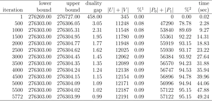
Table 4 shows the result for the problem DavgC provided by Pedings based on the same data as DsumC. The difference is that the cost matrix consists of fractional cost coefficients. We stopped the computation after 5,772 iterations when the duality gap reduced to less
500 1000 1500 2000 iteration 276 200 276 300 276 400 276 500 276 600
Upper and Lower Bounds
Figure 2: Upper and lower bounds vs iteration
500 1000 1500 2000 iteration 20 40 60 80 100
Percentage of Pegged Variables
Figure 3: Percentage of pegged variables vs iteration
than one. The final incumbent may not be optimal, however, more than 95% of variables were pegged.
We solved the problem Judges100 in Charon and Hudry [7]. It assumes that 50 judges rank 100 candidates. Each judge prefers i to j with a probability 0.5 + 0.35(j− i)/(n − 1); if he does not prefer i to j, he prefers j to i. The cost coefficient cij is the difference between
the number of judges preferring i to j and the number of judges preferring j to i. See c(1)ij of (2.1). We solved the linear programming relaxation of the problem. The optimal value, denote by ωupLP, of the linear programming relaxation is the smallest possible value of the upper bound that the Lagrangian relaxation could provide. We set the iteration limit to 10,000 in the proposed algorithm and solved ten instances. In Table 5 the column %0 gives the ratio (ωup− ωLPup)/ωupLP in percent to show how close ωup is to ωupLP. The column
“relative duality gap” shows that a narrow duality gap still remains, and it prevents the proof of optimality of the incumbent solution. We compared the proposed algorithm and Xpress Optimizer 21.01.06 run on a PC with an Intel Core i7, 2.80GHz processor and 6 GB of memory. The column %3 shows the ratio of the best incumbent value obtained by the proposed algorithm and the optimal value. Although our algorithm failed to complete the computation with an optimality proof in most cases, it provided a good lower bound at an
Table 1: Result for DsumC : no pegging test
lower upper duality time
iteration bound bound gap |U| + |V | %1 |P
0| + |P1| %2 (sec) 1 276183.00 276629.00 446.00 345 0.00 0 0.00 0.01 500 276219.00 276221.00 2.00 10410 0.08 0 0.00 2.35 1000 276219.00 276220.00 1.00 10693 0.08 0 0.00 4.91 1500 276219.00 276220.00 1.00 10865 0.08 0 0.00 7.60 2000 276219.00 276220.00 1.00 11016 0.08 0 0.00 10.32 2212 276219.00 276219.00 0.00 11060 0.08 0 0.00 11.48
Table 2: Result for DsumC : ordinary pegging test
lower upper duality time
iteration bound bound gap |U| + |V | %1 |P
0| + |P1| %2 (sec) 1 276183.00 276629.00 446.00 345 0.00 0 0.00 0.01 500 276219.00 276221.00 2.00 10410 0.08 50836 84.68 2.39 1000 276219.00 276220.00 1.00 10693 0.08 54421 90.65 5.08 1500 276219.00 276220.00 1.00 10916 0.08 55076 91.75 7.87 2000 276219.00 276220.00 1.00 11015 0.08 55386 92.26 10.66 2141 276219.00 276219.00 0.00 11073 0.08 55386 92.26 11.40
Table 3: Result for DsumC : improved pegging test
lower upper duality time
iteration bound bound gap |U| + |V | %1 |P
0| + |P1| %2 (sec) 1 276183.00 276629.00 446.00 345 0.00 0 0.00 0.02 500 276219.00 276221.00 2.00 10410 0.08 50836 84.68 2.48 1000 276219.00 276220.00 1.00 10693 0.08 55953 93.21 8.66 1500 276219.00 276220.00 1.00 10882 0.08 56760 94.55 13.16 2000 276219.00 276220.00 1.00 11046 0.08 57156 95.21 17.36 2193 276219.00 276219.00 0.00 11091 0.08 57156 95.21 18.45
Table 4: Result for DavgC : improved pegging test
lower upper duality time
iteration bound bound gap |U| + |V | %1 |P
0| + |P1| %2 (sec) 1 276269.00 276727.00 458.00 345 0.00 0 0.00 0.02 500 276303.00 276306.05 3.05 11248 0.08 47290 78.78 2.28 1000 276303.00 276305.31 2.31 11548 0.08 53840 89.69 9.27 1500 276303.00 276304.95 1.95 11780 0.09 55361 92.22 14.31 2000 276303.00 276304.77 1.77 11948 0.09 55919 93.15 18.83 2500 276303.00 276304.62 1.62 12025 0.09 55930 93.17 23.22 3000 276303.00 276304.45 1.45 12062 0.09 56384 93.92 27.64 3500 276303.00 276304.35 1.35 12089 0.09 56570 94.23 31.88 4000 276303.00 276304.24 1.24 12138 0.09 56747 94.53 35.94 4500 276303.00 276304.15 1.15 12154 0.09 56896 94.78 39.96 5000 276303.00 276304.09 1.09 12171 0.09 56996 94.94 44.06 5500 276303.00 276304.02 1.02 12187 0.09 57122 95.15 47.88 5772 276303.00 276303.99 0.99 12191 0.09 57122 95.15 49.24
early stage and also the pegging test worked well.
Table 5: Result for Judges100
LRPT Xpress
duality relative time optimal time
instance gap duality gap %0 %2 (sec) value (sec) %3
Judges100a 25.00 4.1e-4 3.8e-3 58.71 12.98 60834.00 118.00 99.99
Judges100b 21.00 3.4e-4 4.9e-3 65.45 12.26 61752.00 102.10 99.99
Judges100c 30.00 4.9e-4 6.4e-3 52.26 13.43 60598.00 111.10 99.97
Judges100d 0.00 0.0 0.0 91.45 9.81 61592.00 85.70 100.00
Judges100e 43.00 7.0e-4 9.4e-3 35.84 12.93 61120.00 113.70 99.95
Judges100f 20.00 3.3e-4 4.6e-3 65.11 12.36 60220.00 143.70 99.97
Judges100g 10.00 1.6e-4 4.1e-3 75.23 12.57 60888.00 107.60 99.99
Judges100h 33.00 5.5e-4 1.1e-2 48.99 13.98 60490.00 249.70 99.99
Judges100i 10.00 1.7e-4 1.1e-3 73.09 13.03 60400.00 130.40 99.99
Judges100j 60.00 1.0e-3 1.9e-2 11.70 14.76 59946.00 853.80 99.97
Another problem Median39 in [7] is a 39-item problem made by drawing the orientation of the arc between i and j with a probability 0.5 for each orientation, and choosing its weight randomly from a uniform distribution between 1 and 10. We observe from the column %0 of Table 6 that the Lagrangian relaxation worked well, and the duality gap shrank at an early stage.
Table 6: Result for Median39
LRPT Xpress
duality relative time optimal time
instance gap duality gap %0 %2 (sec) value (sec) %3
Median39a 70.00 2.4e-2 1.7e-1 0.00 7.52 2898.00 257.40 99.34
Median39b 68.00 2.4e-2 1.7e-1 0.00 7.38 2889.00 397.60 99.72
Median39c 44.00 1.5e-2 8.0e-2 0.00 7.46 2966.00 169.80 99.87
Median39d 54.00 1.8e-2 1.1e-1 0.00 6.54 2958.00 245.00 100.00
Median39e 51.00 1.8e-2 8.9e-2 0.00 7.86 2868.00 243.00 100.00
Median39f 83.00 2.9e-2 4.2e-2 0.00 8.60 2905.00 404.00 99.72
Median39g 80.00 2.8e-2 8.2e-2 0.00 7.50 2900.00 1282.70 99.93
Median39h 94.00 3.3e-2 1.1e-1 0.00 8.27 2878.00 2784.70 99.83
Median39i 71.00 2.5e-2 9.0e-2 0.00 7.41 2902.00 489.20 99.90
Median39j 63.00 2.2e-2 1.1e-1 0.00 7.05 2860.00 397.90 99.90
The first two problems DsumC and DavgC stem from the real-world data, and Judges100 imitates them. The proposed algorithm works successfully for those problems. We observe from the column %0 of Tables 5 and 6 that the Lagrangian relaxation gives an upper bound which is very close to the one provided by the linear programming relaxation. This shows the potential that the Lagrangian relaxation could replace the linear programming relaxation in the branch-and-bound algorithm. The problems we solved are so limited that more well-organized experiments should be carried out before any conclusion is made.
Acknowledgment
We thank anonymous referees for their valuable comments, and Mikael Call, Link¨oping University, Sweden, for drawing our attention to the paper [19].
References
[1] I. Ali, W.D. Cook, and M. Kress: On the minimum violation ranking of a tournament. Management Sciences, 32 (1986), 660–672.
[2] K.J. Arrow: Social Choice and Individual Values (John Wiley and Sons, New York, 1951).
[3] A. Belloni and A. Lucena: Lagrangian heuristics for the linear ordering problem. In: M.G.C. Resende and J.P. de Sousa (eds.): Metaheuristics: Computer Decision-Making (Kluwer Academic Publishers, Dordrecht, 2004), 37–63.
[4] G. Bolotashvili, M. Kovalev, and E. Girlich: New facets of the linear ordering polytope. SIAM Journal of Discrete Mathematics, 12 (1999), 326–336.
[5] V. Campos, F. Glover, M. Laguna, and R. Mart´ı: An experimental evaluation of a scat-ter search for the linear ordering problem. Journal of Global Optimization, 21 (2001), 397–414.
[6] E. C¸ ela: The Quadratic Assignment Problem: Theory and Algorithms (Kluwer Aca-demic Publishers, Dordrecht, 2010).
[7] I. Charon and O. Hudry: A branch-and-bound algorithm to solve the linear ordering problem for weighted tournaments. Discrete Applied Mathematics, 154 (2006), 2097– 2116.
[8] I. Charon and O. Hudry: A survey on the linear ordering problem for weighted or unweighted tournaments. A Quarterly Journal of Operations Research, 5 (2007), 5–60. [9] S. Chanas and P. Kobyla´nski: A new heuristic algorithm solving the linear ordering
problem. Computational Optimization and Applications, 6 (1996), 191–205.
[10] J.P. Doignon, S. Fiorini, and G. Joret: Facets of the linear ordering polytope: A unifica-tion for the fence family through weighted graphs. Journal of Mathematical Psychology,
50 (2006), 251–262.
[11] M.L. Fisher: The Lagrangian relaxation method for solving integer programming prob-lems. Management Science, 27 (1981), 1–18.
[12] C.G. Garcia, D. P´erez-Brito, V. Campos, and R. Mart´ı: Variable neighborhood search for the linear ordering problem. Computers and Operations Research, 33 (2006), 3549– 3565.
[13] A.M. Geoffrion: Lagrangian relaxation for integer programming. Mathematical Pro-gramming Study, 2 (1974), 82–114.
[14] S.T. Goddard: Tournament rankings. Management Science, 29 (1983), 1385–1392. [15] C.G. Gonz´alez and D. P´erez-Brito: A variable neighborhood search for solving the
lin-ear ordering problem. MIC’2001 - 4th Metaheuristics International Conference (2001), 181–185.
[16] M. Gr¨otschel, J. J¨unger, and G. Reinelt: A cutting plane algorithm for the linear ordering problem. Operations Research, 32 (1984), 1195–1220.
[17] M. Gr¨otschel, J. J¨unger, and G. Reinelt: Facets of the linear ordering polytope. Math-ematical Programming, 33 (1985), 43–60.
[18] J.G. Kemeny and J.L. Snell: Mathematical Models in the Social Sciences (Blaisdell, New York, 1972).
[19] T. Larsson, M. Patriksson, and A.-B. Str¨omberg: Conditional subgradient optimization — Theory and applications. European Journal of Operational Research, 88 (1996), 382– 403.
[20] J. Leunga and J. Lee: More facets from fences for linear ordering and acyclic subgraph polytopes. Discrete Applied Mathematics, 50 (1994), 185–200.
[21] J.E. Mitchell and B. Borchers: Solving real-world linear ordering problem using a primal-dual interior point cutting plane method. Annals of Operations Research, 62 (1996), 253–276.
[22] J.E. Mitchell and B. Borchers: Solving linear ordering problems with a combined in-terior point/simplex cutting plane algorithm. In H. Frenk, K. Roos, T. Terlaky, and S. Zhang (eds.): High Performance Optimization (Kluwer Academic Publishers, Dor-drecht, 2000), 349–366.
[23] A. Newman and S. Vempala: Fences are futile: on relaxations for the linear ordering problem. In K. Aardal and B. Gerards (eds.): Integer Programming and Combinato-rial Optimization, Lecture Notes in Computer Science, 2081 (Springer-Verlag, Berlin Heidelberg, 2001), 333-347.
[24] K. Pedings, A.N. Langville, and Y. Yamamoto: A minimum violations ranking method. to appear in Optimization and Engineering.
[25] G. Reinelt: The Linear Ordering Problem: Algorithms and Applications (Helderman, Berlin, 1985).
[26] R. Sedgewick: Algorithms in C, 3rd Edition (Addison-Wesley, Boston, 2002).
Noriyoshi Sukegawa
Graduate School of Systems and Information Engineering University of Tsukuba
1-1-1 Tennodai, Tsukuba Ibaraki 305-8573 Japan