MARKOV MODULATED FLUID QUEUES WITH BATCH FLUID ARRIVALS

Journal of the Operations Research Society of Japan

Vol. 44, No. 4, December 2001

MARKOV MODULATED FLUID QUEUES WITH BATCH FLUID ARRIVALS

(Received November 15, 2000; Revised May 15, 2001)

Abstract In the conventional Markov modulated fluid queue, the buffer content process has a continuous sample path. T h i s paper concerns a Markov modulated fluid queue whose buffer content process may have jumps. T h i s model extends not only the conventional fluid queue but also tlie MAP/G'/l model We give a procedure to get a Laplare-Stieltjes transform of t,lie stationary joint distribution of tlie buffer content and barkground state. Some numerical example;-! are prosetit t d a^i well

1. Introduction

H i e conventional fluid queue is an input-output system of fluid with a buffer. Suppose that input and output rates change according t o a continuous-time Markov chain with a finite s t a t e space. This model is referred t o as a Markov modulated fluzd queue, and the Markov chain is called a background process. There are many applications for Markov modulated fluid queues. For instance, they are successfully applied t o modern

ATM

systems, where the fluicl flow is interpreted as a packet d a t a stream which is processed by

ATM

switches

Fluid queues liave been studied in the much literature for more than t w e n t y years.

For example, see Anick, Mitra and Sondhi [ I ] , Uaver and Lehoczky 151, Mitra

[7j.

Klwalid iind Stern [ I ] , Kogers [9] and Asiniisseii [3]. In particular, Rogers [9] and Astiiiissen [;i]

r ~ n s i d e r the first, passage time of the hnffer content t o obtain the empty probability and t h e stationary joint distribution of the buffer cont,ent and the background state. They show that I he stationary joint distribution has the matrix-exponential form, which is determined by a ( * m a i n mat rix equation. In Rogers [9], the matrix equation is determined by Wiener-I Iopf factorization. Asmussen [3] directly derives the matrix equation, then solves it by it eration. Furt~hermore, he considers the case t h a t the fluid flow is sub.ject t o Brownian motion

In this paper, we are interested in the ~ i t ~ u a t i o n thai a fluid model has a n extra input

in addition t o the conventional fluid flow. For example, such an input describes very liipli rate arrivals in short periods, e . g , big file transfers from a liigli speed source in i\ telei-oin-

tiiiinieation network. If they infrequently occur, it is natural t o process them together with the conventional fluid t o gain better performance per cost. It may be also natural to have separate buffers for different types of sources. However it would further c ~ m p l i c a t ~ e s an analysis. As the first step, we here concentrate on the t,otal buffer contents, which can be also considered for the separate buffer model. Thus, we extend the Markov modulated fluid

queue in such a way t h a t its input flow may have upward jumps which is determined hy the background Markov chain. We assume t h a t amounts of jumps are independent and identically distributed under given state transitions. We refer t o such jumps as bntch ,fl?/?d

arrf p a l s .

Since our model has a piecewise linear sample path and the background process is Marko- vian, t.he model includes the workload process of the MAP/G'/\ queue, in which services may depend on its arrival process. Here, the workload and t h e arrival process can lie inter- pret,ed as the buffer content and the background process, respectively, in which t,here are no input flow except for jumps and the output flow rates are always 1 . Hasegawa and Takine [12] and Asmussen [2] use iteration approaches with respect t o tlie first passage time t o t1he idle state t n get, the LST (Laplace-Stieltjes transform) of the stationary joint distribution of the workload and the background st ate. Similar approaches can be found for the fluid

queue in Asmussen [3] and fur the G I / P H / l queue in Sengputa [Ill.

The purpose of this paper is t o get the LST of the stationary joint distribution for the buffer content and the background state. Using the rote cotiservation law (e.g., ser

[.^g.

\vi> see tliat tlie problem t o get the LST reduces t o the problem t o obtain the empty buffer probabilities jointly wit,h the background states. We show t,hat the empty probabilit,ies are given by the stationary vector of a rate matrix determined by certain matrix equations. We then introduce a matrix iteration t o solve the matrix equations, and prove that i t converges to tlie rate matrix.

This paper is organized by six sections. In Section 2, we introduce the Markov rnod~ilat~ed

fluid queue wit8h the batch fluid arrivals, and get tlie LIST which includes the empty

~ I I R ~ I .

probabilities as unknown terms. We tlien consider a random time change for simplifying

argument,^ in Section 3, 4 and 5. In Section 3, we consider t h e first passage time t o the empty state. In Section 4 , we introduce a matrix it,eration, and we show tlie main result.

In Section 5, we compute the empty probabilities. In Section 6, we give a11 algorithm t o compute moments of the buffer content. Numerical examples are also given.

In

Appendix, we derive the LST using the rate conservation law.

2. Background Markov Chain and Buffer Process

Let us describe the fluid system by a stochastic process. We first introduce a background Markov chain. To define a transition rat,e matrix of the Markov chain, we introduce some auxiliary notation. Let

S

be a state space of the Markov chain. We assume that

S

is a finite set, and denote the number of elements in >S' by . S . Let C be a S x .S'I-matrix whose diagonal and off-diagonal elements are negative and nonnegative, respectively. Let !)(x) be a 1.5'1 Y I.S'l-inat,rix whose ( 2 , j ) t h element [ D ( X ) ] ~ , is nonnegative and noit-decn'asiiig finu'Lio11

of ,r

>

0 for all i,j

c

5'. Define

IS\

x liS'l-matrix 1) as

where tlie integration is performed in component-wise. We assume t,hat

where

e

is t h e 15'1-clirnensional column vector whose all components are I . We define

Mtj}

t o be a Markov chain with transition rate matrix Cv+D. We assume t h a t

C+

D is irreducible. Since S is finite, there exists a stationary distribution for C

+

D,

which is denoted by

\S\-

dimensional row vector TT i.e

To describe the buffer content mathematically, we next define function 71 :

S

-+

~ ( S ' ) ( C

7?, - {O}). v does not take value 0, but t,he other struct,ure of 71 is not assumed. Function v

specifies increasing or decreasing rates of the buffer content when it is not empty. That is,

if M(t) = i ?

S

and v ( i ) = -2, then the buffer content decrease with rate 2 a t time t. Let Y ( t ) be the accumulated fluids and batch fluids received u p t o time t . T h a t is,

where Bu(i,jl is the amount of the batch fluids when background process

M ( t )

jumps from

i t o j a t time u, and A^ is a counting process of D-type transitions which include transit ions

from any state t o itself. Note t h a t j) is subject t o the distribution [ / ^ ( . r ) ] , , / [ / ? ] , , . Thus, a jump of {Y(t)} only occur by D-type transition of the background process. l?(.r)- type transition is a D-type with a jump amount of {^(it)} which is less than or equal .r. Y(t) may be negative. Then, buffer content process X ( t ) starting with A'(0) is defined by

X ( f )

= Y ( t )

+

1nax{X[0), - inf

Y

(u)}.

O < l l < f

We define 15'1 x

I

S

1

matrices:

V = diag(v(i); i E

S),

l:,,,, --- diag(v(z)

1;

i E

5)

,

where diag(-) denotes a diagonal matrix. Define sets

S+

and > 5 ' as

I

x IS/-matrix A and 16'1-dimensional row vector x are partitioned into

S+

and

S'

sections

in tlie following way.

For convenience, we also define

S

'

1

x 51-matrix A^* and

IS\

x

S ^

1-mat,rix A*+ as

respectively. A * and A * are similarly defined as

\SA

1

x

\S\-

and

\ S

x 1,s-[-matrices, respectively. For the AdAP/(7/1 queue, we put

5'+

=

0,

S

= S ' ,

,4

-= L~ 4

-

.r -=- i ~ - )

V - - I , while, for the conventional fluid queue, we put D ( x ) = 0 and D -== 0.

For an increasing and bounded function f , its IJST (Laplace-St,ieltjes transform) is de-

noted by f

*(0),

and its

LT

(Laplace transform) is denoted by f * * ( 0 ) . T h a t is,

Note t h a t f *(0)

-

0 f**(0) - f (0-).

Since we are concerned with the ~ t ~ a t i o n a r y distribution of { ( M ( t ) , A'(()

)},

we can assume without loss of generality t h a t

{Y{t}}

has stationary increments. By the well-known result due t o Loynes [6], X ( t ) has a stationary distribution, i.e. X ( t ) is stable, if

FIII~CY' Queues with Batch Inputs 34 7

We assume that

E ( l F ( l ) )

<

0 throughout this paper, and we denote ( A ' ( t ) , ; ! / ( t ) ) in tlie steady st,ate by (X,

M).

We calculate the LST of stationary joint distribution

P(X

<

x,

M

= i). For i E

S

and t

>

0 , define 16'1-dimensional vector F ( x ) as

[ F ( x ) I i = lim P ( X ( t )

<,

x , M ( t ) = i ) -- P ( X

<

x, M = i ) .

t - + m

Proposition 2.1 For

0

>

0 ,

Hence, F * ( Q is given by

This proposition is proved in Appendix. Note that

[F{0)\,

= 0 for i E

.S"

and

[F(O)],

=

P(,Y =- 0 , A4 =

i)

is unknown yet for i  S - . This will be considered in Section 5.

Iii Section 3, 4 and 5, we assume that function v only takes either 1 or -1. This is sufficient for our analysis since we can always reduce the general case t o this simpler case

by a random time change. In fact, let

and consider the joint process { ( X { t ) , M { t ) ) } defined by these matrices and the rate f'unc- lion. Let

TT

be the stationary distribution of

C

+

6.

Since a sojourn time in statjc i 6 AS is unchanged in distribution by this modification, the buffer

_-

content process is stochastically unchanged as well. Since

TT(l<ii,5)

'

(C.'

+

0)

=

i+(C

+

D )

= 0 ,

TT

is proportional t,o 7rl;,1,5.

In a similar way, we get

where

[F

( 0 ) ] , =

P ( % ( o )

= 0 , G ( 0 ) =

i).

Thus, our problem is reduced t o compute

' F

(0). 3. The First Passage Time to The Empty State

As we discussed in Section 2, we could assume that

u ( S )

= { - I , l } . This assumption will be used in Sections 3, 4 and 5. As we shall see, the first passage time to the empty st,ate is a key t o get the empty probabilities jointly with the background states. We consider the

L S T of the first passage time t o the empty state in this section.

Lot r be the first passage time t o the empty state measured from time 0, i.e.,

T = i n f { u

>

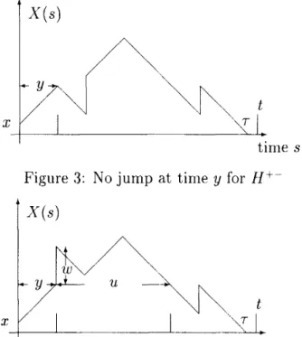
O I X ( u ) = O}.

time s Figure 1: No jump a t time y for

El--

X (s)

Figure 2: A jump a t tAme y for H " -

Clearly, we have / / + ( O l d ) = O t - and

H -

(Old) =

I

.

For

convenience, we introduce the following matrix functions.

'raking t h e LST of these formulas, we have

Lemma 3.1 T h e following equations hold for 6

>

0 and x

>

0.

Prooaf. To derive ( 3 . 3 ) , we first observe the following fact. Given X ( 0 ) = x

>

0 , there is no possibility to attain t h e empty state in time interval [O,

x).

Given X ( 0 ) = 0, i f A'/ ( 0 )

c

S

then T = 0

<,

1. Note t h a t the (i,j)tli element of matrix e c T is a conditional joint probability t h t , in time interval (0, x ] , the buffer content process has no jumps and the liackground process stays in

S

with

M{.r)

Â¥ j , given Af(0) = 2.

If

either the buffer content

process has a jump or the background process enters

S+

in time interval (0, x]

,

we decompose

F111id Queues with Batch Inputs

I

time s Figure 3: No jump a t time y for

H+--

I

time s Figure 4: A jump a t time y for

H^-

buffer content increases due to either a jump or a state change of the background process into

S+.

Let u be the first return time for the buffer content being t o the level a t time y- measured from time if. Thus, time interval (0,

r ]

is partitioned into three sections, the first section is [O, y ) , the second section is [ y , y

+

u ) , and the remaining section is [y

+

u , T ] . These observations yield f - x W - ( d u \ u ) ) H - ' " ( t - y - u \ x - y ) } (Changing variable y to x - y) = l ( x = O ) I -

+

l ( 0

<

x

<

t ) {ec--' t - x - - 1 1 dy _{$ - - ( d u ) H L - ( t} - ( X - y) - u l i , ) } ,

where I ( - ) denotes the indicator function of statement

'.'.

For x

>

0, multiplying e o t t o both sides of (3.5) and integrating from 0 t o oo, we have

Multiplying 0 t o both sides of i t , applying ff"*((Hx) = OH --"(O\x) t,o it, we obtain (3.3) for

x

>

0. This is also valid for x = 0 since

For

77

*

,

we decompose time interval [O, r] into two or three parts. Let y be the first time when either the buffer content has a jump or the background state change into S"-. In the latter case, the time interval is divided into intervals

\0,

y) and [y, r]( see Fip,ure

2).

In

the former case, it is divided into intervals [O, y ) , [y, y 4- u ) and [y

+

u, r], wliere u is the first return time t o level X ( y - ) measured from time y (see Figiire 4). From these observations. we have

(Changing variable y t o y --

x)

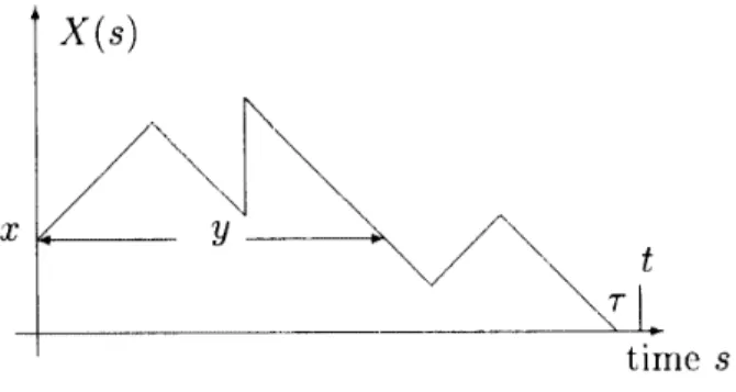
F l ~ ~ i c l Queues with Batch Inputs

Figure 5: T h e another observation for

H ^ -

*t+J--29

/

<

" I @ ^ - - ( d u ) . ll-=o x e 8 ( t - ( y - J;} - - 1 1 ) 11

" ( t

-- ( y -

x)

-- u\y)dydt X)

/

af+a'-2y e - ( G I + + - W ) ( y - - . r ) r - '"@+- ( d u ) 1 0

Multiplying 0 t o both sides of it), we obtain (3.4). D

From Lemma 3.1, we shall derive a matrix exponential form for the LST of 11. To this end, define

Lemma 3.2

Proof. Differentiating both sides of (3.3) with respect t o x yields

a solution of this differential equation is given by (3.6). For (3.7), we need another obser- vation different from Lemma 3.1. We decompose time interval [O, r ] into two parts. Let y

he the first return time t o level .r measured from time

0.

T h e first part is interval (0, y ) and the second part is interval [y,

r ]

(see Figure 5 ) . From these, we have

Multiplying e Ot t o both sides of it and integrating it from 0 t o oo with respert to

t ,

we got

From this equation and (3.6), we obta,in (3.7).

Matrices Q ( 0 ) and / / + * ( 0 [ 0 ) are unknown yet,. We need these matrices at 0 = 0+ to calculate the empty probabilities

F(O)

later. We so define matrices

Q

and

R^

- by

To compute these matrices, we first note the following facts. Lemma 3.3 For 0

>

0, t,he following equations hold.

Proof. From (3.1) and Lemma 3.2, we have

Substituting t,his equation into the definit,ion of Q

( Q ) ,

we obtain (3.9).

On the other hand, differentiating bot,h sides of (3.4) and (3.7), we have

r ~ s p e c t i v ~ l y . (3.2) and Lemma 3.2 imply t,hat,,

From t>his equation, (3.11) and (3.12), we obtain (3.10). D

FluicI Queues with Butch Inputs

Remark 3.1 1. Equations (3.13) and (3.14) can be writdm as:

Recall t h a t we have assumed the case of v ( S ) = {-I, I}. We now rewrite the above equation by the original notation in Section 2. Let,

and change C and D ( x ) t o and D ( x ) in (3.15). Since

6

=

Ki,,C.',

D ( x ) -- _{D ( x )}

and

V

= & / , , s ~ , we have the following expression.

This generalizes a part of the Wiener-Hopf

[9], which is t h e case t h a t

0

= 0, i.e,

fa,ctorization of a Markov chain in Rogers

2. When D = 0, (3.13) and (3.14) are similar t o the corresponding equations in Asmussen

3 . However, they are not the same. T h e reason is t h a t t h e first passage time

of

{Y

( t ) }

t o level 0 starting with Y ( 0 ) = 0 is considered for u(A'/(O))

<

0 in Asniussen [3], while v ( M { 0 ) )

>

0 in this paper, respectively.

3. In the case of the

MAP/G/l

queue, since u ( z ) = - 1 for all

z

E

5,

we can omit (3.14) and terms concerning S+. From (3.13), we have

This is the equation obtained in Hasegawa and Takine [12]. A similar equation is also obtained in Asmussen [ 2 ] .

Definition 3.1 When a matrix has negative diagonal elements and nonnegat,ive

non-diagonal elements, the matrix is called an Mli-matm. (see Seneta [10]).

If

ML-inatrix A satisfies Ae

<^

0, then matrix A is called a subrate matrix. In particular, when .4e = 0,

A is called a rate matrix.

Lemma 3.4 QL- is a rate matrix, i.e.

where

e

is the 5'1-dimensional column vector all of whose elements are 1, and 0 ' is the

Proof.

By t,he definition of

R ^ , R^-

i s obviously a nonnegative matrix. Since

Y

( t )

goes to -oo as

t

tends t o +oo by the stability condition (2.3), r is finite with probability one. Thus, H is the proper joint distribution of r and M ( r ) . Hence,

roo

lim f f ( e \ w ) e =

1

H ( d t \ w ) e - - = e .

(? +0+

I'hus, from (2.1) and (3.13), we have

lini Q ( 0 ) e - = ( 7 - e -

+

C'-'e+

+

D ' ( d w ) lim 11' *(01ii;)e

0 >m 0-^) {

Since

C

is a subra,te matrix and other matrices are nonnegative in t h e right side of (3.13),

Q

also is the ML-matrix. These imply t h a t Q-- is a rate matrix. 0

4. Iteration Algorithm and Its Verification To compute matrices Q and

R^-,

we use iteration. inax{IC.',,];

8

6 S}. Define matrices Q r and

A

'

for 11

2

We choose an q such t h t q

>

0 by

Note t h a t (i) q I + +

+

C'.+'+'

is nonnegative, (ii) it can be shown by induction t h a t

Q ;

and

Hd

- are subrate matrix and substochastic matrix, respectively, and (iii) it is well known

from Perron-Frobenius theorem (for example, see Chapter 2 of Senet,a [lo]) th a t i ) / - - ---

Q,,

is invertible and the inverse matrix is nonnegative. Properties (i), (ii), and (iii) are used later.

T h e next theorem is a key for our c o ~ r ~ p u t a t ~ i o n , which verifies t h a t the it,erations (4.1) and (4.2) indeed converge t o the right values.

Theorem 4.1 For each i )

>

max{]Ci,1; i

e

S}, Q;'

and

R :

are increasing for n and f17;

is nonnegative, and

lim

Qi

- = Q , lini H,! =

R+-.

n+m n+TO (4.3)

Proof. We show the monotonicity of Q ; and

R :

by induction. Since matrices D and (,c-- are n ~ n n e g a t ~ i v e , we have, from (4. I ) ,

Obviously Q [ is an ML-matrix. So, e ^ i and ( r 1 I - Q , ) ' are nonnegative. We then

Fli~id Queues with Hatch Inputs 355

We now assume the m ~ n o t o n i c i t ~ y of Q i and

R :

for k = 0 , 1 ,

...,

n. Then, we get

-- D++

(&W,^"

If' - c^; - l'")

>

0

- .

> r

Since Q,^

>

Q n ,

we obtain

( q I - - -

Q.,

) - - l

<

- (r)I - -

On

the other hand,

(r]I++

+

C ^ + )

is a nonnegative matrix. It follows from these facts t h a t

Thus, we obtain the monotonicity of Q . and

.

By the rnonotonicity of R\ - and

definition R : = O + , we also have the nonnegativity of R^,-.

We next show t h a t Q r ; and

h

'

:

are bounded by

Q--

and

R ' ,

respect,ively. Since

Qi

- Ñ C - and Q - =

C

+

(nonnegative terms), we have Q , i

<

Q . T h e fact,s that,

R,-t

- = 0 7 - and R + is nonnegative matrix yield Ri}

<

R + . Hence, WC have

In a similar way, wo have R:-

<

R1'

. If Qr;'

<

Q--

and R:-

<

R+-, t,llen replacing subscripts 0 and 1 by n and n

+

1 in above equations, respectively, we also have

<

Q-- and R:+~

<

R + . Hence, the inequalities hold true for all n. Thus we have

lirn

<

R+-, lim Q,-

<

Q--.

1tÑ>O M + - O

To complete the proof, we show t h a t

Clearly, (4.4) and (4.5) conclude (4.3). To prove (4.5), we use the uniformization of a Markov chain. Let

{m}

be a uniformized Markov chain obtained from

{M(t)}

with respect t o i n f o l - m rate r ) , let and

N

be a counting process t h a t counts all transition instants of { N t ) } .

356

Obviously, we have

H n ( t \ x )

<

H ( t \ x ) , _rt+m lim H M \ x ) = H(t\x),

G(o\x)

<

W ( 0 \ x ) , _{r t + o c} lim e ( f f \ x ) = H'(01x). Define ISt

1

x IS- I-matrix

@-

and IS-

1

x IS-1-matrix I?;- (x) by

I?:-

= lirn /^-*(010), _{ft;-(x) = lirn H , Ã ‘ ( 0 \ x )}

0 ->0

+

0 > Q {

respective1 y. We then have

We shall prove t h a t

R^-g+-

Â¥II

'

f l ~ ( x ) < c ' - ' - - ~ , -

for all n

>.

0 and all x

>

0. If (4.6) holds, then

R t

<^R[-,

el'--.r

<

(,G-T

-

These inequalities imply

We have (4.5). In what follows, we prove (4.6) by induction on n. 7' ,. ince

from the definitions for n = 0, both inequalities of (4.6) hold for 7~ = 0.

We

assume t h a t these inequalities hold up t o n. We first consider m x ) . Recall t h a t we partition off T into

three sections for H""(t1x) in Section 3. Similarly t o I I ( t \ x ) ^ we partition off r into three sections for

H",^(t\x).

Note t h a t the event for ~ + ~ ( / . l x ) has a t most n

+

1 transitions of the background process. Suppose t h a t M{t) stays in S during time interval (0, x] without jumps for the buffer content process. In this case, there are a t most n

+

1 transitions of the background process. Hence, the corresponding transition probability matrix is not greater than e c .''. If this is not the case, there are ni and n2 sat,isfying 0

<

nl

5

Â¥ rind I

<

Q

<

n

such t h a t the background process has n1 transitions in

S

on the first section [0, y), lias a transition a t time y, has n2 transitions on the second section (y, y

+

u ) , and has a t most

n - 711 - n2 transitions on t h e third section ( y

+

u ,

T\.

From these observations, we have

Fluid Queues with Hatch Inputs

Since we also have

fin'

( u

1

w

)

$

f"fI,^

( d y

\

0 )

fi;

- ( u -- y \w

)

,

we get

Faking t h e limit of the above equation a s 0

-+

0+, and using ( 4 . 1 ) , we have

Hence, it follows from (4.7), (4.8) and the monotonicity of Q7;- on n t h a t

(Integration by parts for

the

first integral)

-

-

(,c--;

{ I - + e-c--- ^;,,-IT _ 1-

}

= ^i.,;^.*

This proves the second inequality in (4.6). It remains t o prove the first inequality in (4.6). For 7/^,l(t10), let y be t h e first time when the uniformiz~d background process { f i ' ~ ( t ) } has a transition. Note t h a t y is exponentially distributed with mean l/r/. Time intlerval 10, r ] is partitioned into three sections: [ 0 , y ) , [ y , y

+

u ) and [ y

+

u ,

r ] ,

where 21 is tlie first return

time of the buffer content t o level X { y - ) measured from time y. Since there is a transition of the uniformized background process a t time y , there are a t most n transitions of tlie uniformized background process on each of time intervals [ 0 , y ) , [ y , y

+

u ) and [ y

+

u , r ] . We define

4;

by

It follows from the above observations t,hat,

From the induction assumption, tlie monotonicity of Q " and the recursion equation (4.2)

Hence, we get

Thus we get ( 4 . 6 ) . This completes the proof. 0

Remark 4.1 T h e iteration ( 4 . 2 ) of

q-

includes a computation of the inverse a t each step

n . When

\ S

is very large, this may be inefficient. We can make another recursion of R:- by

In this algorithm, we only need one inverse operation for

C++

independent of n . Hence, one might think t h a t this recursion is better than the former recursion for a large IS-

1 %

However, our numerical experience shows t h a t this is not always the case (see Table 6.1 in Section

6 ) .

Another problem for this iteration is t h a t it seems hard t o verify its convergence t,o the right values Q-- and

R + .

In particular, we could not prove t h a t

I t :

>

R +

for all n

>

1.

5. The Empty Probabilities

To get the empty probabilities, we first consider busy cycles which is the time interval between successive instants when the buffer content attains 0. We then show t h a t the empty probabilities are given by a stationary vector of

Q--.

Let

x

be a busy cycle length. We define

S

\

x S f - m a t r i x L ( t ) by

Condit,ioning on the first time when the buffer content process leaves the empty state, we have

Hence, we obtain the relationship

/Â¥'11;ic Queues with Hatch Inputs 359

Since the limiting distribution of [ G ' ( t l ~ ) ] , ~ ~ is independent of initial conditions M ( 0 ) = z and

X(0)

= x , we have the following form:

F ( 0 ) is the empty proba,bility vector in the case of v ( S ) = {-I, I}. Lemma 5.1 For 0

>

0 and x

>

0, we have

Proof. We decompose time t into three parts: the first passage time from level x t o the empty state, successive busy cycles and the remaining time up t o time

t .

We then have

where

\S-\

x

IS-

\-matrix LiTi)(y) is the TI,-fold convolution of I, with itself. From (5.1), the

LT

of G ( t 1.r) is

Thus we get (5.2). 0

The following t,heorem gives the representation of F ( 0 ) in the term of the stationary distribution of Q-

,

which always exists because 5"' is finite.

Theorem 5.1 Let K be the stationary distribution of Q . Then,

where Y is the stationary accumulated input process with v(S) = {-I, l}. Proof. Using integration by parts, we have

Multiplying 0 t o ( 5 . 2 ) and taking it in the limit as 6 Ñ> 0+, we have

Thus, we obtain F ( 0 ) Q - - = 0 . Since Q-- is irreducible, which follows froin t,he irre- ducibility of C

+

D , we have

F ( 0 ) - = C K ,

for some constant c

>

0. Multiplying vector e t o both sides of this equation.

To calculate the normalizing constant c, let U + ( t ) be the sojourn time in

S4

up t o time / , and let U ( t ) and U n ( t ) be the sojourn times in

S

u p t o time

t

such that the buffer content is not empty and empty, respectively. Let TYi be the n t h jump instant of

{ X ( t ) } .

Note that,

U+

( t )

+

U , ( t )

+

U; ( t ) =

t ,

N ( t }

0

-5

<

&%bwTn-),

M ( T , , ) )

+

fT+(t) - .f/ ( t )

5

W t ) .

n=l

Since { . Y ( t ) } has the stationary distribution,

Hence, we have

u r n

c = lim - f.-->OG t U + ( t )

U ,

( t ) = 1 - lim(- f ^ ~

t

+-)

t

Let

.EN

denote the expectation by the Palm probability with respect t o N . Substituting t = 1 t o ( 2 . 2 ) and taking the expectation of it, we have

From the stJrong law of large numbers,

Hence we have

n

Thus, combining Proposition 2.1 and Theorem 5.1, we can determine the LST F * ( 0 ) of the stationary joint distribution of

X

and

M .

However, t o get numerical values from tJhis

Finn1 Queues with Hutch Inputs

6. Moments of The Buffer Content and Numerical Examples

We give an algorithm t o compute moments of the buffer content. Wo also exemplify it for some simple cases. We remove the restriction t h a t v ( S ) = { - I , l} in t,his section.

( 2 . 4 ) can be written as:

Let F * ( ' ) ( o ) am1 ~ * ( * ' ) ( f f ) be the kth derivative of

P(O)

and D * ( Q ) , respectively. We note t,hat B ( X v (-1) l ' ~ * ( ~ ) ( o + ) e for k

>

I and F * ( " ) ( o + ) = I T . Differentiating both sides of

(6.1) for r~ times for n

>

1 and taking 0 Ñ 0+ in it, we have

Define 91") and x(") as

Since

r ( e r -

( C

+

D ) ) - '

= I T ,

F*'")

( 0 ) ( e x -

( C

+

D ) ) = ( f 1 7 ' , ) ( 0 ) e ) n

+

g("l,

Differentiating both sides of (6.1) for n+ 1 times for n,

>

1, taking 0

-+

0+ t o it, multiplying

e to the right side of it and applying (6.5) t o it, we have

and, equivalently,

From these calculations, we have the following algorithm: Step 1 . The computation of

F(0)

Step 1-1. Compute stationary distribution TT of C

+

D.

Step 1-2. Compute

c

and . 6 ( x ) .

Step 1-3. Compute Q" by the iteration ( 4 . 1 ) and ( 4 . 2 ) for

C

and

D ( x ) .

Step 1-4. Compute stationary distribution n of Q - - .

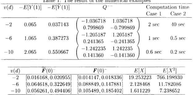
Table 1: The result of the numerical examples

v ( d ) -E\Y(l)] 4 \ Y ( l ) \

Q--

Cornput,ation time

Case 1 Case 2

-2 0.065 - 1 .036718 1.036718 2 sec 40 sec

1.065 -1.205187 1.205187

-6 1 sec 0.5 sec

Step 1-6. Compute Step 2. Compute inverse For k ¥= 1 t,o n : { Step 3-k. Compute Step

4-k.

Compute Step 5-k. Compute St,ep 6-k. F A X k ) = F ( 0 ) by (2.5). matrix of (CTT - ( C

+

D ) )

In the rest of the this section, we consider numerical examples t o show how the algorithm works.

Example 6.1 Suppose t h a t jump sizes are deterministic for each possible transitions. Let B be a

I

S

1

x IS-matrix, whose ( i , j}th element is the jump size of the buffer process when the background state changes from z to j . Define D [ x } by

It

is assumed t h a t

(C

+

D)e

= 0. Then the integral terms in the iteration (1.1) and (4.2)

for Q-- are given by

In a similar way, we can get the integral terms of the iteration for R^". The calculation of

~ * ( * ' ) ( 0 ) for

t

>

1 is given by

Fluici Queues with Batch Inputs 363

where the states are ordered as a , b, c and d . For instance, a

' 5 ' x

15'1-matrix

A

has the

v(d) is varied so as t o represent the heavy traffic case ( - E ( Y ( 1 ) ) close t o zero) and the light traffic case ( - E ( Y ( 1 ) ) far from zero). T h e results are presented in Table 6.1, where for

F ( 0 ) .

F ( 0 ) and Q ,the background states arc ordered as c , d. i.e.,

For those examples, we also compare computation times of both iterations in Section 4 and Remark 4.1, which are referred t o as cases 1 and 2, respectively. Here, numerical results of both iterations are found t o be identical as it is expected.

Acknowledgment T h e author is deeply thankful tm Professor Masakiyo Miyazawa a t Science University of Tokyo for invaluable discussions, and grateful t o anonymous referees for their helpful comments.

References

[ I ] 11. Anick, D. Mitra and M.M. Sondhi: Stochastic theory of a data-handling system with multiple sources. The Bell System Technical Journal, 61-8 (1982) 1871-1894. 21

S.

Asmussen: Ladder heights and the Markov-modulated M / G / l queue. Stochastic

Processes and Their Applications, 37 (1991) 313-326.

[3] S. Asrnussen: Stationary distributions for fluid flow models with or without brownia,n noise. Stochastic Models, 11-1 (1995) 21-49.

[4] A.I. Elwailid and T.E. Stern: Analysis of separable Markov-modulated rate models for information-handling systems. Advances i n Applied Probability, 23 (1991) 105-139. 51 D.P. Gaver and J.P. Lehoczky: Performance evaluation of voiceldata queueing systems.

Applied probability C o m p u t e r Science: the Interface,

I

(1982) 329-346.

[6] R.M. Loynes: T h e stability of a queue with non-independent inter-arrival and service times. Proceedings of Cambridge Philosophical Society, 58 (1962) 497-520.

71

D.

Mitra: Stochastic theory of a fluid model of producers and consumers coupled by a buffer. Advances i n Applied Probability,

20

(1988) 646-676.

8 M. Miyazawa: Rate conservation laws: a survey. Queueing Systems, 15 (1994) 1-58. 9 L.C.G. Rogers: Fluid models in queueing theory and Wiener-Hopf factorization of

[11] B, Sengi~pt~a: Markov processes whose steady state distribution is matrix-exponeritia,l with an applicat,ion t o the G I / P H / l queue. Advances in Applied Probability, 21 (1989)

159-180.

1 2

T.

Takine a,nd T . Hasegawa: The workload in the MAPIG11 queue with sta,t,e- dependent services: Its application t o a queue with preemptive resume priority. Stochas-

tic Models, 10-1 (1994) 183-204.

Appendix. Proof of Proposition 2.1

To calculate the stationary equation of

F ( x ) ,

we assume t h a t X ( t ) and M ( t ) are jointly stationary, and define Z ( t ) as

Z ( t ) = <^"<w^hf(t) = i ) , for each z G S and 0

>

0.

We uniformize { M ( t ) } with rate A given by

Namely, state transition instants are subject t o the Poisson process with rate A , and a t each i s t a n t , the state of M ( t ) changes according t o the transition probability matrix PC 4-

P D ,

where

For P'-transition, jumps are associated. Each jump size is subject t o distribution [ J . ( x ) ] , ~ / ' [ / ? ] , , . We denote the Poisson process by A .

We apply the rate conservation law (see Miyazawa [ 8 ] ) t o Z ( t ) with uniformized

M(t}.

where

E\

is the Palm expectation with respect t o point process A.

To calculate tlie left side of rate conservation law, we have

d d

-Z(t)

= - 0 - ~ ( t ) c - ' " ' ( ~ ) ! ( ~ f ( t ) = i ) .

d t d

t

If X ( t ) = 0 and i E S

',

then X 1 ( t ) = 0. In the other case, we have X ' ( t ) = v(i), Hence, we have

This yields

E ( Z ' ( 0 ) ) = -0v(i)[F*(0)],

+

0 v ( i ) l ( i

c

,S-)[F(0)],.

We calculate tlie right side of (A.1). Because transition instants of the uniformizecl process constitute the Poisson process with rate

A ,

we can apply PASTA t o E A ( 7 ( 0 - ) ) , is(*.

F11/ic! Queues with Batch Inputs We have

A E * ( Z ( ~ - ) )

=

M ( Z ( 0 ) )

=

A[F*(e)]i,

AEA(Z(O+))

=

A E N ( ~

- Ã ˆ . i ( o + ) i ( ~ . f ( O + =

i))

= A ~ E N ( ~

-Èx(Oil

( M ( 0 + )

= z ,

M(0-)

= j ) ) jes

Hence, we get the right side of @ . I ) ,

Thus, we obtain

-OF'(O)V

+

OF(0)V

=

-F*(O)(C

+

D*(O)).

This proves Proposition 2.1.

Hiroyuki Takada

Science University of Tokyo Chiba, Noda 2641, Japan