Vol. 55, No. 3, September 2012, pp. 199–208
A MATHEMATICAL PROGRAMMING APPROACH TO THE MULTI-ROUND TOPOLOGY CONSTRUCTION PROBLEM
IN WIRELESS SENSOR NETWORKS
Mihiro Sasaki Takehiro Furuta Fumio Ishizaki Atsuo Suzuki Nanzan University Nara University of Education Nanzan University
(Received June 10, 2011; Revised August 10, 2012)
Abstract One of the important issues in wireless sensor networks is how to save power consumption and extend the network lifetime. For this purpose, various network topology construction algorithms have been studied. However, most of them are based on a method repeating single round optimization. In other words, by considering the energy dissipation of sensor nodes only in the next round, a network topology in the next round is constructed in a round-by-round manner. The set of the topology constructions based on such a round-by-round view may be far from the optimal solution to maximize the network lifetime. To address this issue, we take the energy dissipation of sensor nodes over multiple rounds into account, and we consider the problem as a multi-dimensional knapsack problem, which enables us to find optimal network topologies until at least one sensor node exhausts its battery power. We also propose a solution method to maximize the network lifetime. The computational experiments show that the proposed approach provides efficient topology construction in the wireless sensor network in terms of network lifetime compared to the cluster-based approach.
Keywords: Telecommunication, wireless sensor network, topology construction,
multi-dimensional knapsack problem
1. Introduction
Wireless sensor networks have been paid much attention due to recent rapid advances of wireless technology combined with prospects of their future progress in scientific, medical, commercial, military areas and so on. A wireless sensor network consists of wireless sensor nodes, which contain devices for sensing, wireless communication and information process-ing. Depending on applications, a wide variety of network sizes can be used. In applications such as environmental monitoring, for example, hundreds or thousands of sensor nodes are deployed in a large monitoring field. When sensor nodes are deployed in a field, a network is first organized in ad-hoc manner. After that, sensor nodes can communicate with each other through the network. In many applications including environmental monitoring, data generated at sensor nodes may be delivered to a specific final destination such as a base station (BS) through the network. Using such wireless sensor networks, we can collect in-formation monitored by sensor nodes at the BS without investigating each sensor node one by one. In addition, wireless sensor networks make it possible to monitor events even in a field where people cannot get in.
For wireless sensor networks, various network architectures have been studied so far (e.g., see [7] and references therein). These network architectures can be classified into two types. One is based on a distributed network, where each sensor node makes decisions for
BS
Sensor field CH
Sensor
(a) Cluster-based sensor network
BS
Sensor field Root
Sensor
(b) Tree-based sensor network
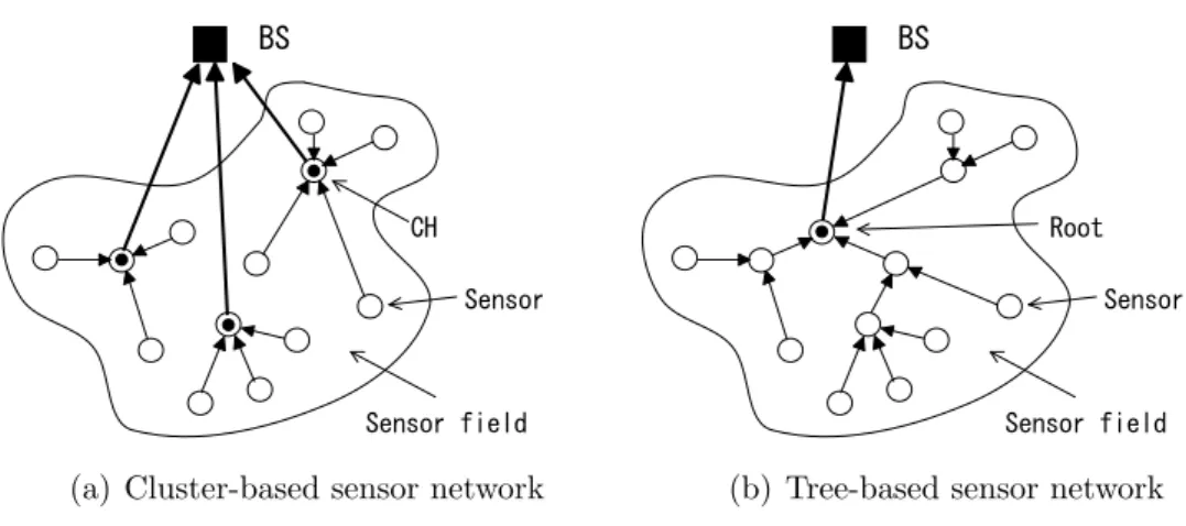
Figure 1: Wireless sensor networks
itself with locally collected information. The other is based on a centralized network, where the BS organizes the network and controls all sensors’ activities. Main advantage of the centralized network is that the BS can collect global information about whole network and sensor nodes, which implies the BS may construct better network topology in order to save power consumption of sensor nodes. Moreover, sensor nodes do not expend their power for network topology construction under the centralized network because the BS which usually has no power limitation is charged with doing all computing. For instance, Heinzelman et al. [4] proposes LEACH-C (Low Energy Adaptive Clustering Hierarchy Centralized), which is considered as a centralized version of LEACH (Low Energy Adaptive Clustering Hierarchy) [3] and they report that LEACH-C is more efficient than LEACH in terms of energy efficiency. Thus, a centralized network is considered as an attractive choice if the BS can construct a good network topology in a practical computational time.
One of crucial challenges in constructing network topology for sensor networks is energy efficiency, because the battery capacities of sensor nodes are severely limited and replacing the batteries is not practical. Once all sensor nodes drain their batteries, the sensor network does not work anymore. Since sensor nodes expend a large amount of energy during data transmission, the transmission distance is a critical factor to save power consumption. The network topology determines transmission distances between sensor nodes. Therefore, an efficient network topology is a key to save power consumption of sensor nodes and extend the network lifetime. In this context, various topology construction in sensor networks have been studied [5, 7]. Among them, cluster-based network organization (see Figure 1(a)) has been considered as a favorable approach in terms of energy efficiency. In this approach, sensor nodes are organized into clusters, and one sensor node in each cluster is selected as cluster head (CH) to play a special role as transfer point. Moreover, each CH creates a schedule for the sensor nodes within the cluster, which allows the radio components of each non-CH-node to be turned off all times except during its transmit time. The rotation of CHs is also important factor in the cluster-based sensor networks in order to achieve a long network lifetime. Since the BS is generally far away from the sensor field, CHs expend much amount of power for data transmission. Hence, CHs would die quickly if the same node continuously worked as a CH. To resolve this problem, the rotation of CHs among sensor nodes is introduced and as a result, when CHs are rotated, all the clusters (i.e., the network topology) is reconstructed by taking the remaining battery capacities of the sensor nodes and the power consumption of each sensor node for communications in the reconstructed network topology into account.
Topology construction algorithms have been proposed so far, including the cluster-based network organization, (see, e.g., LEACH-C [4], clustering algorithm using facility location theory [1] and references therein) is based on a round-by-round view. More precisely, the BS constructs a single topology using the information about the current remaining battery level distribution of sensor nodes, and topology construction is done for every round. The objective in each topology construction is to maximize the total amount of remaining battery power of sensors after the next data transmission. The set of the topology constructions based on such a round-by-round view may be far from the optimal solution to maximize the network lifetime. In this paper, we study the topology construction problem arising in the centralized sensor networks. To overcome the problem of the topology construction method based on the round-by-round view, we propose a multi-round topology construction method, where we consider the changes of the battery level distribution of sensor nodes over multiple rounds as well as the current remaining battery level distribution of sensor nodes in order to find a better set of topologies.
The remainder of this paper is organized as follows. In Section 2, we briefly describe our model and explain a multi-round topology construction arises in the centralized wireless sensor networks. In Section 3, we formulate the multi-round topology construction problem as a multi-dimensional knapsack problem. We also address a problem to find topology construction to maximize the network lifetime, and propose a solution method. In Section 4, we show the computational results. Finally, we give concluding remarks and mention future works in Section 5.
2. Model Description
In this section, we describe a tree-based centralized wireless sensor network considered in this paper. In the sensor network, there is a special facility called base station (BS) located far from the sensor field as shown in Figure 1(a)(b). Sensor nodes monitor event and generate data periodically. We suppose the aim of the sensor network is to periodically collect all data generated by the sensor nodes at the BS.
The operation of the wireless sensor network is divided into rounds. Each round has two phases, which are a setup phase and a data transmission phase. In the setup phase, the BS determines a network topology consisting of all sensor nodes alive, and the BS informs each sensor node of its parent node (the sensor node which it should send a packet to) and child nodes (the sensor nodes which it should receive packets from). In the data transmission phase, each sensor node monitors events and transmits the data using the determined network topology. Rounds are repeated to monitor events continuously. In the data transmission phase, the generated data is delivered in packet to the BS node through the tree network in the following way: A sensor node having child nodes must wait to send a packet including data generated by itself to its parent node until it receives data from all its child nodes. After receiving data from all its child nodes, the sensor node aggregates all data received from the child nodes and data generated by itself in one packet, and it sends the packet to its parent node. We here assume the perfect aggregation, where all packets received by a sensor node can be combined into one packet. After aggregating all data received from its child nodes, each sensor node transmits the same size of data to its parent node. The transmissions from child nodes to their parent node are repeated until all data generated at sensor nodes are finally collected at the BS.
Once a sensor drains its battery, it never monitor events and transmit data. In addition, all sensor nodes drain their batteries, the sensor network does not work anymore. As a
measure for evaluation of wireless sensor networks, we consider a network lifetime, which is defined as the number of rounds repeated before all sensor nodes die. Since the network topology of a sensor network strongly affects its energy efficiency, we should develop a method to construct an energy efficient network topology, which achieves a long network lifetime.
For the aim of extending the network lifetime or maximizing the number of rounds re-peated while a certain percentage of sensor nodes is alive, various methods for topology construction have been addressed [5]. Most of them are based on a round-by-round algo-rithm, where one topology established by the current remaining battery level distribution. After the current optimal topology is found, remaining battery level distribution is updated in order to find an optimal topology for the next round. Repeating these operations until certain criterion is satisfied, the network lifetime or the number of rounds can be obtained. However, repeating this method does not necessarily provide optimal topologies throughout multiple rounds. On the other hand, in the multi-round topology construction proposed in this paper, we take into account continual changing battery level distribution. We can expect to find better topologies over multiple rounds at a time.
In what follows, we will mention an assumption that we put a limitation on the class of the network topologies constructed by our method. In cluster-based networks, data is transmitted from each sensor node to the BS via a CH (see Figure 1(a)). Thus, the number of hops between each sensor and the BS is at most two. In other words, every data can be transmitted to the BS on a two-level tree. Another possibility is a multi-level tree, where more than two hops may be required to transmit data to the BS (see Figure 1(b)). We call this sensor network as a tree-based sensor network. In the tree-based sensor network, we assume that there is one special node which is connected to the BS. We call this sensor node as a root. Data monitored by each sensor node should be transmitted to the root through the given tree, then the root finally transmits the data to the BS. As we see, more than two hops are required from some sensor nodes to the BS in the tree-based sensor network. As the number of hops increases, power consumption caused by the data reception and aggregation increases while that caused by data transmission decreases. However, since power consumption caused by data transmission is most critical, shorter transmission distances would afford to save power consumption. From these observations, allowing more than two hops from a sensor to the BS, we consider a topology construction problem arise in a tree-based sensor network. A forest composed of several trees can be a candidate. In the forest topologies, more than one sensor node should be connected to the BS. However, from our preliminary test to evaluate energy efficiency of both trees and forests, we confirm that trees are more efficient. This may be caused by a large amount of power consumption during the data transmission from the roots to the remote BS. The perfect aggregation may also help trees be more efficient than forests. We therefore consider only the tree-based network topologies excluding forests.
Note that a tree should be a spanning tree of all sensor nodes to ensure network connec-tivity. Once a tree to be used in a round is given, the transmission routes from each sensor node to the BS are uniquely established. Hence, we can compute the power consumption of each sensor node in the round. From these observations, we consider an approach where we first prepare some candidate trees which consists of a spanning tree and a root, then find out which candidate tree should be used how many rounds in order to maximize the number of rounds. This approach enables to construct the optimal set of network topologies for multiple rounds at a time.
3. Formulation and Solution Method
In the following, we show a mathematical programming formulation of the multi-round topology construction problem. First, we employ the following notations.
N : the index set of sensor nodes, T : the index set of candidate trees,
bj: the remaining battery level of sensor node j∈ N,
cij: energy dissipation of sensor j ∈ N when tree i ∈ T is used.
We further introduce xi (i∈ T ) as integer variables, which express the number of rounds
us-ing candidate tree i∈ T . Hence, the multi-round topology construction problem MRTC(N, T ) can be formulated as the following multi-dimensional knapsack problem.
[MRTC(N, T )] maximize ∑ i∈T xi (3.1) s.t. ∑ i∈T cijxi ≤ bj, j ∈ N, (3.2) xi ∈ Z, i∈ T.
The objective (3.1) is to maximize the number of rounds. Constraints (3.2) show that sensor node j ∈ N cannot expend energy over the remaining battery level bj. This problem
is generally NP-hard in the strong sense excluding some special cases [6].
Before we solve MRTC, we need to generate a set of candidate trees. There are some possible ways to generate a set of candidate trees. For example, Tanaka et al. [10] presented a sophisticated approach to generate a set of candidate trees using column generation method. However, here we simply employ the minimum spanning tree and shortest path trees as the candidate trees, and obtain an exact optimal solution of MRTC using an optimization software. The detailed algorithm to solve MRTC used in our computational experiments is described in Section 4.
We further propose a simple algorithm to maximize the network lifetime using MRTC as a subproblem. Note that the optimal objective value of MRTC(N, T ) denotes the maximum number of rounds until at least one sensor node among N drains its battery. Some wireless sensor network systems are rather interested in maximizing the network lifetime. In this case, the network lifetime can be computed in the following manner. First, we solve MRTC(N, T ) with all sensor nodes set N and associated T . After that, we reconstruct the sensor node set N by removing the dead sensor nodes and remake candidate trees set T to be adjusted to the updated N . With the updated N and T , we solve a MRTC(N, T ) again. Repeating these operations until all sensor nodes die, i.e. N =∅, or the optimal value of MRTC(N, T ) becomes 0, we can obtain the network lifetime of the sensor network. Note that we call a sensor is dead if its remaining battery level is not sufficiently large to receive and transmit data. However, it is generally difficult to determine which sensors really do not have enough remaining battery level because the energy dissipation depends on network topologies to be used. Hence, we introduce criteria to determine whether a sensor node is dead. Depending on the criterion, the optimal value of MRTC(N, T ) might be 0 even though N ̸= ∅. We summarize the algorithm to compute the network lifetime as follows.
[Algorithm for computing the network lifetime]
(Input) N : the index set of all sensor nodes. (Output) L: the total number of rounds.
T∗: the set of used trees.
Step 0: (Initialize) Set k := 1, Nk:= N, L := 0 and T∗ =∅.
Step 1: (Tree set-up) Create the set of candidate trees Tk for sensor node set Nk. Set M :=|Tk|. Let tik (i = 1,· · · , M) denote an element of Tk.
Step 2: (Solve) Find an optimal solution x of MRTC(Nk, Tk) with the optimal value zk.
If zk= 0, then go to Step 4.
Step 3: (Update)
(a) Set L := L + zk and i := 1.
(b) If xi > 0, then update T∗ := T∗∪ tik and set fi := xi. If i < M , then set i := i + 1.
Go to Step 3(b).
(c) Update bj := bj −
∑
i∈Tk
cixi. Let D be the index set of the dead sensor nodes. Set k := k + 1, and Nk := Nk−1\D. If Nk is not empty, then go to Step 1.
Step 4: (Terminate) L is the network lifetime which is established by using tree ti ∈ T∗
for fi rounds (i = 1,· · · , |T∗|).
This algorithm also can be regarded as a kind of myopic method, because it doesn’t neces-sarily take into account continual change of remaining battery level distribution throughout the network lifetime. However, as far as the authors know, topology construction considering multiple rounds at a time has never addressed. It may be possible to provide better topolo-gies compared to those provided by the algorithm based on round-by-round optimization such as proposed in [1].
4. Computational Experiments
We made computational experiments to see how long our approach can extend the network lifetime compared to that achieved by the cluster-based approach proposed in [1]. We adopted the same physical constants and parameters as used in [1, 4]. That is, we assume that initial battery level of each sensor node is 0.5 J, i.e. bj = 0.5 for all j ∈ N; energy
dissipation cij is computed under the conditions that the data amount transmitted by each
sensor node is 4200 bits; the electronics energy is 50 nJ/bit; the amplifier energy is 10 pJ/bit/m2 if the transmission distance is less than 87 m and 0.0013 pJ/bit/m4 otherwise; the energy dissipation for data aggregation is set as 5 nJ/bit.
We used an optimization software Xpress-MP (2005B) to solve the problems. All exper-iments were run on a PC with Intel Pentium 4 processor (2.53GHz) and 512MB RAM.
We prepared three test data sets (data1, · · · , data3), where 100 sensor nodes are ran-domly deployed in a 100-meter-square. For convenience, we define the lower left of the square as (x = 0, y = 0) and the upper right of the square as (x = 100, y = 100). We assume that the BS is located at (x = 50, y = 175). These settings are also the same as those used in [1, 4].
In this section, we suppose that the path loss exponent in the path loss model is equal to 2.0 [2, 8, 11], which determines the power consumption of data transmission between sensor nodes. Considering that the distance is measured by squared distance, we selected the minimum spanning tree (MST) and shortest path trees (SPT) as the candidates of the sensor network topology. They are suitable to save the power consumption because they connect the sensor nodes so as to minimize the distance measures. Hence, the set of candidate trees T in our experiments consists of a hundred SPT-based trees and a hundred MST-based trees. For SPT-based trees, we select a sensor node as a root and find the shortest path form the root to all sensor nodes, where the distance is measured by the squared distance. For MST-based trees, we first constructed the MST of the sensor node
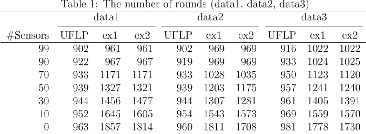
Table 1: The number of rounds (data1, data2, data3)
data1 data2 data3
#Sensors UFLP ex1 ex2 UFLP ex1 ex2 UFLP ex1 ex2
99 902 961 961 902 969 969 916 1022 1022 90 922 967 967 919 969 969 933 1024 1025 70 933 1171 1171 933 1028 1035 950 1123 1120 50 939 1327 1321 939 1203 1175 957 1241 1240 30 944 1456 1477 944 1307 1281 961 1405 1391 10 952 1645 1605 954 1543 1573 969 1559 1570 0 963 1857 1814 960 1811 1708 981 1778 1730
set, where the distance is also measured by squared distance. Then, we created the hundred MST-based trees so that each has a different root. Note that topology of all MST-based trees is the same and each MST-based candidate tree has the different energy dissipation because the root is different.
The objective of the problem is to select the trees from the candidate trees and decide how many rounds we should use the trees so as to maximize the number of rounds until at least one sensor node dies. After that, at least one sensor node can not send data using any given candidate trees. To continue the monitoring, we need to decide new candidate trees without the dead sensor nodes. To remove the dead senor nodes, we need to know whether a sensor node still have enough battery power.
We can consider various criteria for enough battery power of sensor node. If a sensor node has only the power to transmit data to the nearest sensor but it does not have the power to receive data from sensor nodes, the sensor node can not play a role as a relay node in the network. Therefore we consider such sensor nodes as sensor nodes which do not have enough power in our criteria. Also, by considering the power to receive data from multiple sensor nodes instead of a single sensor node, we take safety side criteria for practical use. More specifically, we prepare the set of dead sensor nodes D according to the following two criteria in our experiments. The first is whether a sensor node has enough power to receive data from at least two sensor nodes and transmit the aggregated data to the nearest sensor node. We use this criterion in the first experiment (ex1). The second is whether a sensor node has power to receive data from at least three sensor nodes and transmit the aggregated data to the nearest sensor node. We use this criterion in the second experiment (ex2). Note that the power consumption of receiving and aggregating data is dependent on only the amount of data.
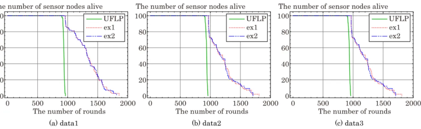
Table 1 and Figure 2 show the comparisons of the number of rounds in the two exper-iments mentioned above and “UFLP” using data1, data2 and data3. The column labeled “UFLP” denotes the results of Furuta et al. [1] which is one of the cluster-based approaches. The number of total rounds in our proposed method is about twice of the number of rounds displayed in “UFLP”. The ex1 provides better results compared to those achieved by the ex2. This can be caused by the different criteria introduced to determine the dead sensor nodes. The criterion introduced in the ex2 is more strict than that of the ex1. Regardless of the strict criterion, the number of dead sensor nodes is the same in both the ex1 and the ex2 at the beginning. However, as the rounds are repeated, more sensor nodes can be regarded as dead in the ex2. After all, the ex1 which has rather soft criterion tends to provide better results.
(a) data1 0 500 1000 1500 2000 0 20 40 60 80 100
The number of rounds The number of sensor nodes alive
ex1 UFLP ex2 (b) data2 0 500 1000 1500 2000 0 20 40 60 80 100
The number of rounds The number of sensor nodes alive
ex1 UFLP ex2 (c) data3 0 500 1000 1500 2000 0 20 40 60 80 100
The number of rounds The number of sensor nodes alive
ex1 UFLP ex2
Figure 2: Relationship between the number of sensor nodes alive and the number of rounds Table 2: The cumulative number of data transmissions
data1 data2 data3
# rounds UFLP ex1 ex2 UFLP ex1 ex2 UFLP ex1 ex2 900 90000 90000 90000 90000 90000 90000 90000 90000 90000 1000 — 99484 99484 — 99238 99255 — 100000 100000 1100 — 107713 107713 — 105894 105990 — 108266 108299 1200 — 115120 115120 — 111213 111309 — 114804 114729 1300 — 121558 121558 — 115119 115043 — 119769 119683 1400 — 126290 126143 — 117264 117108 — 123845 123210 1500 — 129424 129445 — 118770 118750 — 126152 125348 1600 — 131237 131319 — 119758 119863 — 127420 126274 1700 — 132125 132066 — 120381 120563 — 128137 126786 1800 — 132484 132580 — 120581 — — — — 1900 — — — — — — — — —
In addition to the comparisons of the number of rounds, we focus on the total number of data transmissions throughout the network lifetime. Table 2 shows the cumulative numbers of data transmissions for the case after 900 rounds in each instance. Since no sensor node drains its battery before 900 rounds in any instance, those numbers before 900 rounds are exactly the same as the number of rounds times 100. We observed that our proposed method increases the total number of transmissions by 1.4 to 1.5 times compared to the UFLP-based method.
Table 3 reports the CPU time. The row labeled “# Solved MRTC” shows how many multi-round topology construction problems were solved to obtain the network lifetime. Next two rows show average and maximum CPU time for a MRTC, respectively, and the last row shows the total CPU time computed by the number of solved MRTC times average CPU time. Although the maximum CPU time for a MRTC seems to depend on instances, we obtained the solutions in a small amount of time.
These results show that our algorithm provides energy-efficient selection of the spanning trees throughout the network lifetime in a reasonable time. As a result, the network lifetime is drastically extended.
5. Conclusion
We consider a multi-round topology construction problem arises in the centralized wireless sensor networks, and formulated the problem as a multidimensional knapsack problem. We
Table 3: CPU time
data1 data2 data3 ex1 ex2 ex1 ex2 ex1 ex2 # Solved MRTC 60 55 57 46 45 36 Average CPU time (sec.) 4.0 4.7 1.0 1.2 1.5 1.6 Maximum CPU time (sec.) 184 184 4 6 4 4 Total CPU time (sec.) 240.0 258.5 57.0 55.2 67.5 57.6
made computational experiments to compare our results with those provided by the previous approach using the cluster-based network. The computational experiments show that the number of rounds until at least one sensor node drains its battery is larger than those achieved in the previous study. The experiments also shows that the network lifetime is also extended about two times of the previous results. Our solution method provides better results in a reasonable time.
In this paper, in order to extend the network lifetime of wireless sensor networks, we focus on the topology construction which is energy efficient. However, although the delivery rate of data to the BS is an important factor in the topology construction of wireless sensor networks as well as energy efficiency, we do not consider the delivery rate of data. As a future work, we will develop a topology construction method considering both the delivery rate and energy efficiency. Since the failure of data transmission randomly occurs in wireless networks, we may need the analysis of a mathematical model incorporating the stochastic characteristics of the failure process.
Acknowledgment
The authors are grateful to the anonymous referees for their helpful comments and sugges-tions. This research was supported by Grant-in-Aid for Scientific Research (B) (grant No. 21310098) and (C) (grant No. 22510162) from Japan Society for the Promotion of Science.
References
[1] T. Furuta, M. Sasaki, F. Ishizaki, A. Suzuki, and H. Miyazawa: A new clustering model of wireless sensor networks using facility location theory. Journal of the Operations Research Society of Japan, 52 (2009), 366–376.
[2] A. Goldsmith: Wireless Communications (Cambridge University Press, 2005).
[3] W.R. Heinzelman, A. Chandrakasan, and H. Balakrishnan: Energy-efficient commu-nication protocol for wireless microsensor networks. Proceedings of the 33rd Hawaii International Conference on System Sciences (2000).
[4] W.B. Heinzelman, A.P. Chandrakasan, and H. Balakrishnan: An application-specific protocol architecture for wireless microsensor networks. IEEE Transactions on Wireless Communications, 1 (2002), 660–670.
[5] J.C. Hou, N. Li, and I. Stojmenovic: Topology construction and maintenance in wireless sensor networks. In I. Stojmenovic (ed.): Handbook of Sensor Networks: Algorithms and Architectures (John Wiley & Sons, 2005), 311–341.
[6] S. Imahori, Y. Miyamoto, H. Hashimoto, Y. Kobayashi, M. Sasaki, and M.Yagiura: The complexity of the node capacitated in-tree packing problem. Networks, 59 (2012), 13–21.
[7] M. Kochhal, L. Schwiebert, and S. Gupta: Self-organizing of wireless sensor networks. In J. Wu (ed.): Handbook on Theoretical and Algorithmic Aspects of Sensor, Ad Hoc Wireless, and Peer-to-Peer Networks (Auerbach Publications, 2006), 369–392.
[8] T.S. Rappaport: Wireless Communications Principles and Practices (Prentice-Hall, 2002).
[9] M. Sasaki, T. Furuta, F. Ishizaki, and A. Suzuki: Multi-round topology construction in wireless sensor networks. Proceedings of the Asia-Pacific Symposium on Queueing Theory and Network Applications (2007), 377–384.
[10] Y. Tanaka, S. Imahori, M. Sasaki, and M. Yagiura: An LP-based heuristic algorithm for the node capacitated in-tree packing problem. Computers & Operations Research,
39 (2012), 637–646.
[11] D. Tse and P. Viswanath: Fundamentals of Wireless Communication (Cambridge Uni-versity Press, 2005).
Mihiro Sasaki
Department of Information Systems and Mathematical Sciences
Nanzan University
27 Seirei, Seto, Aichi 489-0863, Japan E-mail: [email protected]