Vol. 59, No. 1, January 2016, pp. 72–109
PH FITTING ALGORITHM AND ITS APPLICATION TO RELIABILITY ENGINEERING
Hiroyuki Okamura Tadashi Dohi
Hiroshima University
(Received September 2, 2015; Revised December 21, 2015)
Abstract This article presents parameter estimation of phase-type (PH) distribution. PH distribution is widely used in model-based performance evaluation such as reliability and queueing system, and is defied by an absorbing continuous-time Markov chain (CTMC). Since non-Markovian model can be approximated by a CTMC by replacing general distributions with PH distributions, the parameter estimation is a challenging issue in stochastic modeling. We focus on the statistical inference algorithms to estimate not only the parameters of PH distribution with grouped, truncated and missing data but also the probability density function, and give two examples of PH fitting in reliability engineering.
Keywords: Reliability, phase-type distribution, maximum likelihood estimation, EM
algorithm, transient analysis, continuous-time Markov chain
1. Introduction
Stochastic models are frequently used for evaluation of system performance indices in
queue-ing and reliability analyses. In particular, dynamic system behavior of computer
sys-tems, telecommunication network syssys-tems, or production syssys-tems, is described as a state-dependent stochastic process. In such model-based performance evaluation, discrete-time and continuous-time Markov chains (DTMCs/CTMCs) are quite popular to model the sys-tem behavior [12]. The time-homogeneous DTMC and CTMC are mathematically tractable and can provide both stationary and transient system performance indices through analyti-cal approaches. However, when some of state transitions are represented by non-Markovian-type distributions such as Weibull, normal, log-normal distributions, it becomes difficult to take analytical approaches in many cases. In such cases, although Monte-Carlo (MC) sim-ulation approach may be practically useful in some situations, it may not be often suitable when the high accuracy of system indices is required. For example, in reliability analysis of mission-critical systems, five through nine nines of quantitative reliability are demanded in practice. Hence, the analytical approach, if possible, is more preferred to simulation approach in quantitative reliability assessment.
Phase-type (PH) distribution is defined for a non-negative random variable which is an absorbing time on time-homogeneous DTMC or CTMC process. It is known that the stochastic model described by PH distributions is reduced to a time-homogeneous Markov process with DTMC or CTMC. Furthermore the PH distribution can get close to any prob-ability distribution with any precision if the number of states of the underlying DTMC or CTMC infinitely increases [5]. This property provides advantages to both approxima-tion and estimaapproxima-tion in model-based performance analysis. For example, PH expansion is regarded as one of the most useful approximation techniques for non-Markovian models, where non-Markovian-type distributions are replaced by PH distributions under the
situ-ation where the probability density function (p.d.f.) or cumulative distribution function (c.d.f.) of Markovian-type distribution is known. PH expansion approximates the non-Markovian models to Markov models which are analytically tractable, and the PH-expanded Markov model approximates the non-Markovian model accurately if the number of states of the underlying DTMC or CTMC is appropriate. In the estimation, even though the true distribution is unknown, PH distribution is expected to be close to the true distribution
when the number of states of the underlying DTMC or CTMC infinitely increases∗. That
is, by assuming that the true distribution is a family of PH distributions, we develop a non-parametric-like estimation approach.
In both cases, key issues are how to determine the appropriate number of states of the underlying DTMC or CTMC and how to determine parameters of PH distributions. These are called the PH fitting problem. The article mainly focuses on the second issue, i.e., how to determine PH parameters when the number of states of the underlying DTMC or CTMC is fixed. Since the essential difference between approximation and estimation is whether we know the p.d.f. or c.d.f. of the true distribution or not, PH approximation is used to indicate the PH fitting when the p.d.f. or c.d.f. of the true distribution is known. On the other hand, PH estimation means the PH fitting when we do not know the true distribution. Furthermore, the terminology, PH fitting, is used when it is not necessary to distinguish whether we know the true distribution or not in the article.
Since PH distributions generally involve a large number of parameters, PH fitting is not so tractable. In past, there are two major approaches for PH fitting with moments and Kullback-Leibler (KL) divergence. The former determines PH parameters so as to fit theoretical moments of PH distribution to moments from samples or p.d.f. In PH estimation, the moments are estimated from samples. In PH approximation, the moments are calculated from the p.d.f. of distribution. On the other hand, KL-based PH fitting is to find PH parameters that minimize KL divergence from a PH distribution to the true distribution. In the context of PH estimation, this corresponds to maximum likelihood (ML) estimation of PH distribution.
This tutorial article presents a survey of PH fitting and introduces the state-of-the-art PH fitting algorithm for PH distributions defined on CTMC presented by [67]. More specifically, we give KL-based PH approximation and estimation procedures with the EM (expectation-maximization) algorithm [17, 87] and uniformization technique. We also refer to the numerical tool implemented with the statistical software R. Further, we give two examples of PH fitting; PH estimation for software reliability assessment and PH approxi-mation for dynamic reliability modeling based on a Markov regenerative process (MRGP). We introduce the so-called phase-type software reliability model (PH-SRM) [59, 60, 63] and mention how to use the PH estimation algorithm to the parameter estimation of PH-SRM. In the second example, we apply the PH approximation (PH expansion) to describe a par-allel system with single repair facility by means of the MRGP and evaluate the pointwise availability.
The organization of this article is as follows. In Section 2, we describe the mathematical definition and properties of PH distribution. Section 3 overviews PH fitting and introduces an efficient ML estimation algorithm when grouped, truncated and missing data are given. In Section 4, we formulate PH-SRM in the context of software reliability engineering, and present how to use the PH estimation algorithm to get model parameters of PH-SRM. Section 5 demonstrates the PH apporximation of MRGP. We describe the definition of ∗In practice, the bias of estimates should be considered.
MRGP and provide the Kronecker representation of the approximate MRGP. Finally, we conclude the article with future research directions of PH fitting in Section 6.
Abbreviation and acronym
PH: Phase type
CTMC: Continuous-time Markov chain DTMC: Discrete-time Markov chain MC: Monte-Carlo
p.d.f.: probability density function c.d.f.: cumulative distribution function KL: Kullback-Leibler
ML: Maximum likelihood EM: Expectation maximization MRGP: Markov regenerative process
PH-SRM: Phase-type software reliability model APH: Acyclic PH GPH: General PH CF1: Canonical form 1 CF2: Canonical form 2 CF3: Canonical form 3 LS: Laplace-Stieltjes
AIC: Akaike information criterion BIC: Bayesian information criterion MM: Moment matching
LLF: Log-likelihood function
MCMC: Markov chain Monte Carlo
IID: independent and identically distributed NA: Not available
MAP: Markovian arrival process SRM: Software reliability model
NHPP: Non-homogeneous Poisson process CPH-SRM: PH-SRM with CF1
HEr-SRM: PH-SRM with hyper-Erlang distribution GO: Goel-Okumot model
ISS: Inflection S-shaped model
Q-R ISS: Quasi-renewal time-delay model based on ISS Beta-Mix: NHPP-based SRM with beta mixture
MSE: Mean squared error MLL: Maximum log-likelihood DF: Degrees of freedom
EXP: Exponential (transition) GEN: General (transition) DE: Double exponential WEI: Weibull distribution LOG: Log-normal distribution CV2: Squared coefficient of variation
2. PH Distribution
2.1. Definition
The PH distribution is defined as a probability distribution for time to absorption in a time-homogeneous CTMC with an absorbing state. Without loss of generality, we consider an absorbing CTMC on the finite state space{1, 2, . . . , m, m+1} with the following infinitesimal generator: QP H = ( T τ 0 0 ) , (2.1)
where the state m + 1 indicates the absorbing state. Also, T is an infinitesimal generator between transient states {1, 2, . . . , m}, and τ is a column vector for transition rates to the absorbing state. Let τi and λi,j denote the i-th entry of τ and the (i, j)-entry of T , respectively. By using the column vector 1 whose all elements are 1, the vector τ is given
by τ =−T 1. The above absorbing CTMC process is called a phase process, denoted by Jx
where x indicates time, and the transient state of phase process is called phase in general. The PH random variable is defined by the first passage time to the absorbing state on the phase process Jx, i.e.,
X = inf{x ≥ 0; Jx = m + 1}. (2.2)
Suppose that the initial phase J0 is determined by a probability (row) vector α =
(α1, . . . , αm) over the transient states. Then the p.d.f. and c.d.f. of X can be written with the PH parameters (α, T , τ ): †
fP H(x) = α exp(T x)τ , 0≤ x < ∞, (2.3)
FP H(x) = 1− α exp(T x)1, 0 ≤ x < ∞, (2.4)
respectively.
2.2. Properties
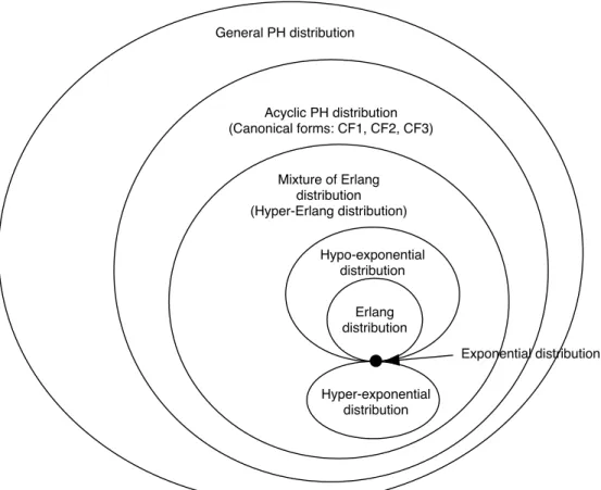
It is known that PH distribution consists of the mixture/convolution of exponential distri-butions. Hence it involves some well-known probability distributions as the special cases. The exponential distribution is the simplest PH distribution when the number of phases (the number of transient states in the phase process) is 1. Similarly, since the Erlang distribution, hyper-exponential distribution, hypo-exponential distribution and mixture of Erlang distri-butions can be obtained from the mixture/convolution of exponential distridistri-butions, they are also subclasses of PH distributions. These subclasses do not have any cyclic structure between transient states, and then belong to a class of acyclic PH distribution (APH). Since the APH distribution is mathematically tractable and a superclass of commonly-used dis-tributions such as the exponential and Erlang disdis-tributions, the APH distribution is quite important in applications. Also the PH distribution whose parameters do not have any constraint is called the general PH distribution (GPH). The relationship among subclasses of PH distributions is summarized in Figure 1.
Cumani [16] derived three canonical forms of APH distribution; CF1, CF2 and CF3, and proved that all of APH distributions can be reconfigured to any one of the canonical forms †In fact, since the PH representation (α, T , τ ) is redundant, the PH distribution is essentially defined only
by (α, T ). In our PH fitting, it is noted that the diagonals of T are computed from non-diagonals of T and
Erlang distribution Hypo-exponential distribution Mixture of Erlang distribution (Hyper-Erlang distribution) Acyclic PH distribution (Canonical forms: CF1, CF2, CF3) General PH distribution Exponential distribution Hyper-exponential distribution
Figure 1: Relationship among subclasses of PH distributions
which have 2m− 1 free parameters. Specifically, CF1 (canonical form 1) is defined by
α =(α1 α2 · · · αm ) , (2.5) T = −β1 β1 −β2 β2 . .. . .. −βm−1 βm−1 −βm , τ = 0 .. . 0 βm , (2.6)
where 0 < β1 ≤ · · · ≤ βm. Throughout the article, blanks in a matrix indicate zero entries. When the parameter constraint 0 < β1 ≤ · · · ≤ βm does not hold in Equation (2.6), the resulting PH distribution is called a bidiagonal PH distribution [28] to distinguish it from CF1.
On the other hand, CF2 and CF3 are given as variants of CF1. Concretely speaking, by using CF1 parameters, CF2 can be represented in the form;
α = (1 0 · · · 0), (2.7) T = −βm α1βm α2βm · · · αm−1βm −β1 β1 . .. . .. −βm−2 βm−2 −βm−1 , τ = αnβn 0 .. . 0 βm−1 . (2.8)
Also, CF3 is given by α =(1 0 · · · 0), (2.9) T = −βm (1− γm)βm −βm−1 (1− γm−1)βm−1 . .. . .. −β2 (1− γ2)β2 −β1 , τ = γmβm .. . γ2β2 γ1β1 , (2.10) where γi = αi/(1 − ∑m
l=i+1αl). When the parameter of CF3 are allowed to be complex numbers, the structure of CF3 reduces Coxian distribution [19,85]. That is, CF3 is a special case of Coxian distribution in which the parameters are restricted to be real numbers.
PH distribution has closure properties for convolution, mixture, minimum and
maxi-mum operations. Let XA and XB be independent PH random variables with parameters
(αA, TA, τA) and (αB, TB, τB), respectively. Then XC = XA+ XB becomes a PH random variable with the following parameters:
• convolution αC = ( αA 0 ) , TC = ( TA τAαB TB ) , τC = ( 0 τB ) . (2.11)
A mixture of XA and XB is expressed as XC = χXA+ (1− χ)XB where χ is the indicator random variable with probability p. This means the random variable XC chooses either of
XA or XB with probability p. The random variable XC becomes a PH random variable
having the parameters: • mixture αC = ( pαA (1− p)αB ) , TC = ( TA TB ) , τC = ( τA τB ) . (2.12)
In a fashion similar to the previous discussion, let XCmin = min(XA, XB) and XCmax =
max(XA, XB) be minimum and maximum of XA and XB, respectively. Then they are PH
random variables with the following parameters: • minimum αC = αA⊗ αB, TC = TA⊕ TB, τ = τA⊗ 1 + 1 ⊗ τB, (2.13) • maximum αC = ( αA⊗ αB 0 0 ) , TC = TA⊕ TB τAT⊗ I I ⊗ τB B TA , τ = τ0B τA , (2.14)
where ⊗ and ⊕ are the Kronecker product and sum, respectively.
Furthermore, let X1, . . . , Xn be independent PH random variables. Then we suppose that ˜XA and ˜XB are random variables that are generated by convolution, mixture, mini-mum and maximini-mum operations of X1, . . . , Xn. According to the above properties, ˜XA and
˜
System failure
1 2 3 2 4
failure A failure B Component faiure
AND gate
OR gate
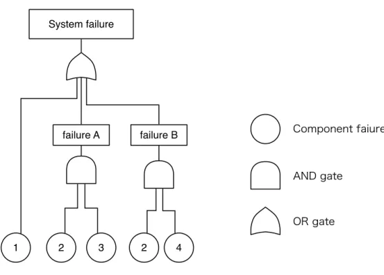
Figure 2: An example of fault tree
that a random variable generated by convolution, mixture, minimum and maximum opera-tions of ˜XA and ˜XB becomes a PH random variable generated by independent PH random variables X1, . . . , Xn. Thus, although the expressions of p.d.f. are more complex, the closure properties hold even in the class of ˜XA and ˜XB.
In the reliability engineering, it is commonly supposed that a system failure is caused by multiple component failures. This causal relationship is often modeled by fault trees. The fault tree analysis is a kind of root-cause analysis which represents the condition that causes an event occurrence by using AND/OR conditions [7]. Figure 2 illustrates an example of fault tree. In this tree, leaf nodes correspond to component failure events, and AND/OR gates express the failure conditions for upper events. The AND gate means that the upper event occurs only when all the leaf events occur. The OR gate indicates that the upper event occurs when at least one event occurs.
In AND gate, XA and XB denote random variables of event occurrence time for lower
events A and B. Then the upper event occurrence time is given by max(XA, XB). Similarly, in the case of OR gate, the upper event occurrence time is given by min(XA, XB). That is, the top event occurrence time is given by min-max operations of component failure times. In Figure 2, e.g., the system failure (top event) occurs at min(X1, max(X2, X3), max(X2, X4)).
From this insight, when X1, . . . , X4 are mutually independent, we have the following
propo-sition.
Proposition 2.1. In the fault tree model, when component failure times are assumed to
be independent PH random variables, the system failure time also becomes a PH random variable which is constructed by min-max operations of component failure times.
By combining the above proposition with Equations (2.13) and (2.14), it is easily seen that when component failure times follow independent APH random variables, the system failure time also becomes an APH random variable. Furthermore, since any APH distribution can be transformed to the canonical forms, we have the following proposition.
Proposition 2.2. In the fault tree model, when component failure times are assumed to
be independent APH random variables, the probability distribution of system failure time is expressed as the canonical forms.
This property implies that even if we do not know the exact failure mechanism for the system failure such as fault trees, the system failure time distribution is represented by a canonical form of PH distributions. In particular, since component failure times are often independent exponential random variables in the reliability engineering, the canonical forms are appropriate for representing the probability distribution of system failure time.
3. PH Fitting
3.1. Historical survey
The purpose of PH fitting is to determine PH parameters (α, T , τ ) so as to approximate the target distribution by the fitted PH distribution. In particular, the PH estimation is the PH fitting from data under the situation where we do not know the true distribution and the PH approximation is the PH fitting from p.d.f. or c.d.f. of the true distribution. In both cases, the accuracies of estimation and approximation depend on the number of phases and the subclasses. For example, if the number of phases is 1, the corresponding PH distribution is the exponential distribution. Needless to say, the exponential distribution does not possess the relatively high fitting ability. Hence we encounter the following three research questions on PH fitting:
(i) What is the appropriate subclass of PH distributions? (ii) How many phases are required?
(iii) How should the estimates of (α, T , τ ) be determined?
On the research question (i), three kinds of phase structures, GPH, APH and mixture of exponential/Erlang distributions, are typically used. In particular, since APH distribution can be transformed to the canonical forms, PH fitting for APH distribution is discussed in the context of parameter estimation of canonical forms.
It is worth mentioning that the research question (ii) has been still open as an unre-solved problem for PH fitting. Several approaches have been proposed in past researches. Particularly, in the PH approximation, the number of phases is determined by the criterion of approximation. For example, when the criterion is given by the moments of a target distribution, the accuracy of approximation can be defined by how many moments should be used. Osogami and Harchol-Balter [71] and Bobbio et al. [10] gave the moment-based method for APH distribution with the first three moments, and revealed the minimum number of phases that is necessary to match the first three moments. A more sophisticated approach is based on the Laplace-Stieltjes (LS) transform. O’Cinneide [54–57] discussed the characteristics of PH distribution, and provided the lower bounds on the number of phases of PH distribution by means of poles of LS transform. He and Zhang [28] derived the phase reduction algorithm to find the minimal representation of Coxian distribution based on O’Cinneide’s works. On the other hand, in the PH estimation, the theoretically valid approach in the sense of statistics would be to use information criteria such as AIC (Akaike information criterion) [2] and BIC (Bayesian information criterion) [78]. They are used in many applications of statistical model selection problem. The information criterion essentially handles the penalty term incurred by increasing the number of model param-eters. That is, this method leads to find the appropriate number of phases by means of information criteria.
On the research question (iii), there are many variations proposed in the past literature, where the methods can be classified into three types. The first method is moment-based approach, which is often called moment matching (MM) method and is mainly used in the PH approximation. The concept of MM method is to find PH parameters so that the population moments can fit the moments derived from samples or p.d.f. of the true distribution. As mentioned before, the accuracy of MM method depends on how many moments is used. In general, it is difficult to develop the MM method with a large number of moments. In fact, many authors focused on only the first two or three moments to determine PH parameters.
The main concern for the earliest PH fitting was the MM method with special structure such as a mixture of Erlang distributions and CF3 with 2 phases using the first two mo-ments in application of Markov model [48]. Altiok [4] presented a method to approximate general distributions by PH distributions via LS transform of the mixture of exponential distributions. van der Heijden [85] gave a simple formula for the MM method of CF3 with the first three moments. Aldous and Shepp [3] showed that the number of phases is easily determined by the coefficient variation for Erlang distribution. Johnson and Taaffe [34–37] and Johnson [33] conducted several works on PH fitting for the mixture of Erlang distribu-tions with non-linear programming techniques in terms of the difference of p.d.f. as well as moments. In the context of the MM method for APH distribution, Telek and Heindl [80] presented a method for 2-phase APH distributions. Osogami and Harchol-Balter [71] and Bobbio et al. [10] proposed the MM methods that provide the minimum number of phases to fit to the first three moments. van de Liefvoort [84] and Telek and Horvath [81] extended the PH distribution to the matrix-exponential distribution, and discussed the MM methods with high-order moments. In PH fitting, the problem of how to approximate a heavy-tailed distribution was often discussed. The heavy-tailed distributions are distributions whose tails are not exponentially decayed. Feldmann and Whitte [20] discussed the method to approximate the heavy-tailed distribution with the mixture of exponentials.
Here we remark on the computational risk in the use of MM method in the PH estimation. It has no doubt that the MM method works well for PH approximation, because moments are exactly computed from the p.d.f. However, in the PH estimation, we should always consider the estimation errors for moments. In general, an estimate of high-order moment is rather sensitive to errors caused by random samples. Thus it is difficult to obtain the accurate estimates of high-order moments when the number of samples is small. In addition, there is the situation where we cannot know even the first moment exactly in the case where some data are missing.
The second approach is to use KL (Kullback-Leibler) divergence which is called KL-based approach in this article. The KL-KL-based approach reduces the maximum likelihood (ML) estimation when we do not know the true distribution. The ML estimation is a commonly used technique to estimate model parameters by maximizing the likelihood so that the observed data are drawn from the model. The advantage of ML estimation is that it can estimate parameters from any type of data and can enjoy several rich properties in statistics, such as asymptotic normality in PH fitting. Then this approach is superior to the moment-based approach in the PH estimation. Also, when we know the p.d.f. of the true distribution, the KL-based approach is to determine PH parameters that minimizes the KL divergence to the true distribution. Since the KL divergence is defined by the integral of the true distribution and a PH distribution, the KL-based approach is also used in the PH approximation through techniques of numerical quadrature. On the other hand, since the computation cost of KL-based approach is relatively high compared to moment-based
approach, the challenging issue is to reduce the computation cost. The EM (expectation-maximization) algorithm [17, 87] is frequently used for PH fitting.
Bobbio and Cumani [9] presented the ML estimation for canonical forms by solving the non-linear programming. In their method, the linear programming was iteratively applied to solve the non-linear programming to maximize the log-likelihood function (LLF). The method was almost similar to the steepest decent method but introduced constraints to ensure the parameter constraints of canonical forms. Also Bobbio and Telek [11] carried out experiments on ML estimation for APH distribution. Asmussen et al. [6] proposed an EM algorithm for GPH distribution, and also presented an idea of using numerical quadra-ture for PH approximation. Olsson [70] extended the EM algorithm for PH estimation with censored data. Okamura et al. [66] improved Asmussen’s EM algorithm with respect to time complexity of the number of phases. Also, they proposed an improved algorithm for estimating APH distribution with EM algorithm. Moreover, in [67], the PH fitting with EM algorithm is extended to handle grouped, truncated and missing data. On the other hand, for PH fitting with the mixture of Erlang distributions (hyper-Erlang distribu-tion), Thummler et al. [82] and Panchenko and Thumler [72] developed the EM algorithms which can determine the phase structure of hyper-Erlang distribution. Compared to APH distribution, the hyper-Erlang distribution is inferior to representation ability because the hyper-Erlang distribution is a sub-class of APH distribution. However, their algorithm is much faster than the EM algorithms for APH distributions. Based on the EM algorithms for hyper-Erlang distributions, Reinecke et al. [77] proposed the method to combine the data clustering and PH fitting to fit to heavy-tailed distribution according to the idea of Feldmann and Whitte [20].
The third method is Bayes estimation, which is only used for the PH estimation. In the Bayesian paradigm, it is assumed that unknown model parameters are random variables. By observing field data, the corresponding probability distribution of model parameter is updated according to the Bayes theorem. The updated probability distribution of model parameter is called the posterior distribution, and the probability distribution of model parameter before the update is called the prior distribution. The main feature of Bayes estimation is to compute the posterior distributions of parameters. The Bayes estimation enables us to evaluate not only interval estimation of parameters but also the predictive distribution in many cases. However, the computation of posterior distribution is often more expensive than moment-based and KL-based approaches as well.
Bladt et al. [8] proposed an MCMC (Markov chain Monte Carlo) algorithm for GPH dis-tribution with Markov jump process to approximate the posterior disdis-tributions. Watanabe et al. [86] considered an improved MCMC algorithm by using the uniformization technique to improve the computation speed. Yamaguchi et al. [92] and Okamura et al. [68] pro-posed the variational Bayes algorithms for the mixture of Erlang distributions and GPH distribution. The presented methods are much faster than MCMC-based algorithms.
3.2. KL-based PH fitting
The KL-based approach is to determine PH parameters that minimize KL divergence. Con-sider the situation where a p.d.f. f (x) is approximated by a PH distribution with p.d.f. fP H(x). The KL divergence KL(f, fP H) between f (x) and fP H(x) is defined as follows.
KL(f, fP H) = ∫ ∞ 0 f (x) log f (x) fP H(x) dx = ∫ ∞ 0 f (x) log f (x)dx− ∫ ∞ 0 f (x) log fP H(x)dx. (3.1)
The KL divergence means the distance between f (x) and fP H(x). If f (x) and fP H(x) are ex-actly same, the KL divergence becomes 0. Since the first term of Equation (3.1) is a constant with respect to the PH parameters, we find fP H(t) maximizing
∫∞
0 f (x) log fP H(x)dx.
In the PH estimation, since the true distribution f (x) is unknown, we estimate the second term of Equation (3.1) from observed data. For example, let x1, . . . , xnbe IID (independent and identically distributed) samples from the true distribution. The second term can be estimated as the following LLF:
∫ ∞ 0 f (x) log fP H(x)dx≈ n ∑ i=1 log fP H(xi), (3.2)
and the PH parameters are determined to solve the maximization problem the above LLF. In the PH approximation, the p.d.f. of the true distribution is known. When applying a suitable numerical quadrature to the second term of Equation (3.1), we have
∫ ∞ 0 f (x) log fP H(x)dx≈ n ∑ i=1 wilog fP H(xn). (3.3)
The above equation implies that the KL-based PH approximation reduces the ML esti-mation with the weighted IID samples (x1, w1), . . . , (xn, wn). Also, the accuracy of PH approximation is evaluated by the KL divergence between them.
3.3. EM algorithm
The EM algorithm is an iterative method for ML estimation under the situation where there exists unobserved data [17, 87]. Let D and U be observable and unobservable data vectors, respectively, and we estimate a model parameter vector θ from only the observable data D. Then the problem corresponds to finding a parameter vector that maximizes a marginal LLF: ˆ θ = argmax „ L(θ; D), (3.4) L(θ; D) = log p(D; θ) = log ∫ p(D, U; θ)dU, (3.5)
where p(·) is a probability density or mass function.
From Jensen’s inequality, for any model parameter vector θ′, we have L(θ; D) = log ∫ p(D, U; θ)dU = log ∫ p(D, U; θ) p(U|D; θ′)p(U|D; θ ′)dU ≥ ∫ p(U|D; θ′) log p(D, U; θ) p(U|D; θ′)dU ≡ Z(θ; θ ′). (3.6)
Since the distribution of unobservable data is
p(U|D; θ) = ∫ p(D, U; θ)
the lower bound of the marginal LLF Z(θ; θ′) can be rewritten by Z(θ; θ′) =∫ p(U|D; θ′) logp(U|D; θ)
∫
p(D, U; θ)dU
p(U|D; θ′) dU
= ∫
p(U|D; θ′) log p(U|D; θ)
p(U|D; θ′)dU + log ∫
p(D, U; θ)dU. (3.8)
Then we have the following formula:
L(θ; D) − Z(θ; θ′) = KL(p(U|D; θ′), p(U|D; θ)). (3.9)
Also the difference L(θ; D) − L(θ′;D) holds
L(θ; D) − L(θ′;D) = Z(θ; θ′)− Z(θ′; θ′) + KL(p(U|D; θ′), p(U|D; θ)). (3.10)
Since KL(·, ·) ≥ 0, the model parameter vector θ that satisfies Z(θ; θ′)− Z(θ′; θ′) > 0 yieldsL(θ; D) − L(θ′;D) > 0. In other words, when we find θ that maximizes Z(θ; θ′) for a fixed θ′, the marginal LLF for θ is greater than that for θ′.
Let Q(θ|θ′) denote the expected LLF of the complete data vector (D, U) with respect to the distribution for unobservable data vector under a provisional parameter θ′, i.e.,
Q(θ|θ′) = ∫
p(U|D; θ′) log p(D, U; θ)dU. (3.11)
Then the lower bound Z(θ; θ′) is rewritten in the form:
Z(θ; θ′) = Q(θ|θ′)−∫ p(U|D; θ′) log p(U|D; θ′)dU. (3.12)
Since the second term of the above equation is constant with respect to θ, we obtain Z(θ; θ′)− Z(θ′; θ′) = Q(θ|θ′)− Q(θ′|θ′). Thus the maximization of Z(θ; θ′) is reduced to the maximization Q(θ|θ′).
According to the above discussions, the EM algorithm consists of E-step and M-step. E-step computes the expected LLF Q(θ|θ′) with a given provisional parameter vector θ′. In the M-step, we find a new parameter vector θ that maximizes the expected LLF:
θ ← argmax
„
Q(θ|θ′). (3.13)
Since the marginal LLF for θ is surely greater than that for θ′, we can perform the same
E- and M-steps by replacing θ′ with θ. These steps are repeatedly executed until the
parameters converge. It should be noted that the EM algorithm does not guarantee that the parameters converge to ML estimates. That is, the EM algorithm may converge to a local maximum of the marginal LLF. To avoid the convergence to a local maximum, it is important to choose appropriate initial guesses of parameters.
3.4. PH estimation with grouped, truncated and missing data
Here we introduce a PH estimation algorithm proposed by [67] based on ML estimation with EM algorithm. It can be applied to estimating GPH parameters with grouped, truncated and missing data.
The grouped data consists of several time intervals and the number of events that occur in the time intervals. The time points that generate time intervals are called break points
Table 1: Examples of grouped, truncated and missing data for PH fitting (break points: 0, 10, 20, . . . , 90, 100)
Data (a) Data (b)
Time interval The number of events
[0, 10] 1 [10, 20] NA [20, 30] 4 [30, 40] 10 [40, 50] NA [50, 60] 30 [60, 70] 10 [70, 80] 12 [80, 90] 4 [90, 100] 0 [100,∞] 5
Time interval The number of events
[0, 10] 1 [10, 20] NA [20, 30] 4 [30, 40] 10 [40, 50] NA [50, 60] 30 [60, 70] 10 [70, 80] 12 [80, 90] 4 [90, 100] 0 [100,∞] NA
in this article. Table 1 (a) presents an example of the grouped, truncated and missing data on break points 0, 10, 20, . . . , 100. In this table, the values in intervals [10, 20] and [40, 50] are missing and denoted as NA (not available). Furthermore, the bottom row means that 5 samples are truncated at 100. Similarly, Table 1 (b) gives another example. In this case, several samples are truncated at 100 but we cannot know the exact number of truncated samples. In this way, it is worth noting that the incomplete data such grouped, truncated and missing data frequently appear in field data analysis.
Consider the grouped data on the break points 0 = x0 < x1 < · · · < xK, i.e., the data consist of the number of samples for K + 1 intervals [0, x1), [x2, x3), . . . , [xK,∞). For the sake of notational convenience, let X(k,l) be the l-th sample in the k-th interval. In addition, we assume two kinds of intervals; observable and unobservable intervals. LetI and I be the sets of indexes of observable and unobservable intervals. Note thatI and I are disjoint, and
that I ∪ I gives all the indexes, i.e., I ∪ I = {1, 2, . . . , K + 1}. We can count the numbers
of samples in only the observable intervals, but the numbers of samples in the unobservable intervals are unknown, i.e., the data are missing in the unobservable intervals.
LetD = {nk}k∈I be the numbers of samples in observable intervals. Define the following
unobserved variables:
• Uk: the number of samples in the k-th unobserved interval [xk−1, xk), k∈ I.
• B(k,l)
i : an indicator random variable for the event that the phase process of X(k,l) begins with phase i.
• Z(k,l)
i : the total sojourn time of phase i on the phase process of X(k,l).
• Y(k,l)
i : an indicator random variable for the event that the phase process of X(k,l) is i just before the absorption.
• M(k,l)
i,j : the total number of phase transitions from i to j on the phase process of X(k,l). Since the estimates of CTMC parameters are given by frequencies and sojourn time for each state under the situation where the CTMC process is completely observed, the M-step
formulas of PH parameters are obtained from Equation (3.13) in the following: αi ← ∑ k∈IE [∑nk l=1B (k,l) i ¯¯¯ D ] +∑k∈IE[∑Uk l=1B (k,l) i ¯¯¯ D ] ∑ k∈Ink+ ∑ k∈IE[Uk|D] , (3.14) τi ← ∑ k∈IE [∑nk l=1Y (k,l) i ¯¯¯ D ] +∑k∈IE[∑Uk l=1Y (k,l) i ¯¯¯ D ] ∑ k∈IE [∑nk l=1Z (k,l) i ¯¯¯ D ] +∑k∈IE[∑Uk l=1Z (k,l) i ¯¯¯ D ] , (3.15) λi,j ← ∑ k∈IE [∑nk l=1M (k,l) i,j ¯¯¯ D ] +∑k∈IE[∑Uk l=1M (k,l) i,j ¯¯¯ D ] ∑ k∈IE[∑nl=1k Z (k,l) i ¯¯¯ D ] +∑k∈IE[∑Uk l=1Z (k,l) i ¯¯¯ D ] . (3.16)
Note that all the expected values are computed by the provisional PH parameters θ = (α, T , τ ).
Next we derive the analytical forms of the expected values in Equations (3.14)–(3.16). Since it is known that the posterior distribution of unobserved samples U = {Uk}k∈I be-comes a negative multinomial distribution [49], the expected value of Uk, k ∈ I becomes the similar expression of the expected value of negative multinomial distribution:
E[Uk|D] = N∫xk xk−1fP H(x)dx ∑ i∈I ∫xi xi−1fP H(x)dx , k ∈ I, (3.17)
where N =∑k∈Ink, and fP H(x) is the p.d.f. of PH distribution.
Define the following row and column vectors for a PH random variable X and its phase process Jx:
[f (x)]i = P (Jx = i), [b(x)]i = P (X = x|J0 = i), (3.18)
where i̸= 0 and, for the sake of notational convenience, P (X = x) means the p.d.f. Since X(k,l) are IID samples, the expected value of B(k,l)
i in the observable interval is
given by E [ n k ∑ l=1 B(k,l)i ¯¯ ¯¯ ¯ D ] = nkE[Bi|xk−1 < X ≤ xk] = nkP (J0 = i, xk−1 < X ≤ xk) P (xk−1 < X ≤ xk) = nk ∫xk xk−1P (J∫ 0 = i)P (X = x|J0 = i)dx xk xk−1P (X = x)dx = nk ∫xk xk−1αi[b(x)]idx ∫xk xk−1fP H(x)dx . (3.19)
In the case of unobservable interval, by using the posterior distribution of Uk, the expected value becomes E [ U k ∑ l=1 Bi(k,l) ¯¯ ¯¯ ¯ D ] = ∞ ∑ n=0 nE[Bi|Uk = n, xk−1 < X ≤ xk]P (Uk= n|D) = ∞ ∑ n=0 n∫xk xk−1αi[b(x)]idx ∫xk xk−1fP H(x)dx P (Uk = n|D) = E[Uk|D] ∫xk xk−1αi[b(x)]idx ∫xk xk−1fP H(x)dx = N ∫xk xk−1αi[b(x)]idx ∑ i∈I ∫xi xi−1fP H(x)dx . (3.20)
Similarly, we have E [ n k ∑ l=1 Yi(k,l) ¯¯ ¯¯ ¯ D ] = nk ∫xk xk−1P (X = x, J − x = i)dx P (xk−1 < X ≤ xk) = nk ∫xk xk−1P (J − x = i)P (Jx = 0|Jx−= i)dx P (xk−1 < X ≤ xk) = nk ∫xk xk−1[f (x)]iτidx ∫xk xk−1fP H(x)dx , (3.21) E [ U k ∑ l=1 Yi(k,l) ¯¯ ¯¯ ¯ D ] = N∫xk xk−1[f (x)]iτidx ∑ i∈I ∫xi xi−1fP H(x)dx , (3.22) where Jx− = limx′→0+Jx−x′.
For Zi(k,l) and Mi,j(k,l), the expected values in the observable interval are
E [ n k ∑ l=1 Zi(k,l) ¯¯ ¯¯ ¯ D ] = nk ∫xk xk−1 ∫x 0 P (X = x, Ju = i)dudx P (xk−1 < X ≤ xk) = nk ∫xk xk−1 ∫x 0 P (Ju = i)P (X = x,|Ju = i)dudx P (xk−1 < X ≤ xk) = nk ∫xk xk−1 ∫x
0[f (u)]i[b(x− u)]idudx
∫xk xk−1fP H(x)dx , (3.23) E [ n k ∑ l=1 Mi,j(k,l) ¯¯ ¯¯ ¯ D ] = nk ∫xk xk−1 ∫x 0 P (X = x, Ju−= i, Ju = j)dudx P (xk−1 < X ≤ xk) = nk ∫xk xk−1 ∫x
0 P (Ju− = i)P (Ju = j|Ju− = i)P (X = x,|Ju = j)dudx
P (xk−1 < X ≤ xk) = nk ∫xk xk−1 ∫x
0[f (u)]∫ iλi,j[b(x− u)]jdudx xk
xk−1fP H(x)dx
. (3.24)
Also the expected values in the unobservable interval become
E [ U k ∑ l=1 Zi(k,l) ¯¯ ¯¯ ¯D ] = N∫xk xk−1 ∫x
0 [f (u)]i[b(x− u)]idudx
∑ i∈I ∫xi xi−1fP H(x)dx , (3.25) E [ U k ∑ l=1 Mi,j(k,l) ¯¯ ¯¯ ¯ D ] = N∫xk xk−1 ∫x
0[f (u)]iλi,j[b(x− u)]jdudx
∑ i∈I
∫xi
xi−1fP H(x)dx
. (3.26)
f (x) = α exp(T x) and b(x) = exp(T x)τ : fk = ∫ ∞ xk f (x)dx = α(−T )−1exp(T tk), (3.27) ˜ fk = ∫ xk xk−1 f (x)dx = fk−1− fk, (3.28) bk = ∫ ∞ xk b(x)dx = exp(T xk)1, (3.29) ˜ bk = ∫ xk xk−1 b(x)dx = bk−1− bk, (3.30) Hk = ∫ ∞ xk ∫ u 0 b(x− u)f(u)dudx = ∫ xk 0
exp(T (xk− u))1α exp(T u)du + 1fk
= Υ + 1fk, (3.31) ˜ Hk = ∫ xk xk−1 ∫ u 0 b(x− u)f(u)dudx = Υk−1− Υk+ 1 ˜fk, (3.32) where Υk = ∫xk
0 exp(T (xk− u))1α exp(T u)du. By using the above vectors and matrices,
the expected values are rewritten as E [ Uk| D] = N α˜bk ∑ i∈Iα˜bi , (3.33) E [ n k ∑ l=1 Bi(k,l) ¯¯ ¯¯ ¯ D ] = nkαi[˜bk]i α˜bk , E [ U k ∑ l=1 B(k,l)i ¯¯ ¯¯ ¯ D ] = ∑N αi[˜bk]i u∈Iα˜bu , (3.34) E [ n k ∑ l=1 Yi(k,l) ¯¯ ¯¯ ¯ D ] = nk[ ˜fk]iτi α˜bk , E [ U k ∑ l=1 Yi(k,l) ¯¯ ¯¯ ¯ D ] = ∑N [ ˜fk]iτi u∈Iα˜bu , (3.35) E [ n k ∑ l=1 Zi(k,l) ¯¯ ¯¯ ¯ D ] = nk[ ˜Hk]i,i α˜bk , E [ U k ∑ l=1 Zi(k,l) ¯¯ ¯¯ ¯ D ] = ∑N [ ˜Hk]i,i u∈Iα˜bu , (3.36) E [ n k ∑ l=1 Mi,j(k,l) ¯¯ ¯¯ ¯ D ] = nkλi,j[ ˜Hk]j,i α˜bk , E [ U k ∑ l=1 Mi,j(k,l) ¯¯ ¯¯ ¯ D ] = N λ∑i,j[ ˜Hk]j,i u∈Iα˜bu . (3.37)
It can be seen that ˜fk, ˜bk, ˜Hk are replaced by fk, bk, Hk, respectively, at k = K + 1, because tK+1 goes to infinity.
Much computation time of the EM algorithm for PH distribution is spent for the calcu-lation of convolution integral of matrix exponential. In [61, 66], the effective computation algorithm for the convolution integral of matrix exponential was proposed based on the uniformization. Let Υ(t; v1, v2) be the convolution integral of matrix exponential;
Υ(x; v1, v2) =
∫ x 0
exp(T (x− u))v1v2exp(T u)du, (3.38)
where v1 and v2 are arbitrary column and row vectors, respectively. Algorithm 1 presents
a pseudo code to compute Υ(x; v1, v2). In this algorithm, ε is an error tolerance for
the computation of Poisson probability. The function PoiBound(µ, ε) gives the first point
where the c.d.f. of Poisson distribution with mean µ becomes more than 1− ε. The
Algorithm 1 Uniformization-based convolution integral of matrix exponential
function convint(x, v1, v2) : return value Υ
r← max(abs(diag(T ))); P ← I + T /r; R ← PoiBound(rx, ε) v1(0) ← v1 for i = 1 : R do v1(i)← P v1(i− 1) end for v2(R) ← PoiProb(R + 1, rx)v2 for i = R− 1 : 0 do v2(i)← v2(i + 1)P + PoiProb(i + 1, rx)v2 end for Υ← 0 for i = 0 : R do Υ← Υ + v1(i)v2(i)/r end for end function
e−µµn/n!. Also I means the identity matrix. The time complexity of Algorithm 1 is
pro-portional to a square of the number of phases. In particular, when T is a sparse matrix, the time complexity is proportional to the number of non-zero elements of T .
Applying the algorithm to the computation of expected values, we define H = K+1∑ k=1 wkH˜k, (3.39) where wk = { nk/π˜bk, k ∈ I, N/∑u∈Iπ˜bu, k∈ I. (3.40) From ˜H = Hk−1− Hk and Hk= Υ(xk; 1, α) + 1fk, we get
H = K+1∑ k=1 wk1 ˜fk+ K ∑ k=1 Υ(∆xk; bk−1, ck), (3.41) where ∆xk = xk− xk−1 and ck = K ∑ l=k (wl+1− wl)α exp(T (tl− tk)). (3.42)
Algorithm 2 indicates our E-step procedure for PH distributions under grouped,
trun-cated and missing data according to the above formulas. In this algorithm, the
func-tion convint(x, v1, v2) denotes the convolution integral of matrix exponential presented
in Algorithm 1. By using the results of Algorithm 2, the parameters are updated as
αi ← αi[B]i/(N + U ), τi ← τi[Y ]i/[H]i,i and λi,j ← λi,j[H]j,i/[H]i,i.
As mentioned before, any APH distribution can be transformed to three types of canon-ical forms [16]. In the M-step, the parameters are updated by using the results of E-step;
αi ← αi[B]i N + U, λi ← λi[H]i+1,i [H]i,i for i = 1, . . . , m− 1, λm ← λm[Y ]m [H]m,m . (3.43)
Algorithm 2 E-step procedure for PH distributions with grouped, truncated and missing data B← 0; Y ← 0; H ← O f0 ← α(−T )−1; b0 ← 1; N ← 0; U ← 0 for k = 1 : K do fk ← fk−1exp(T ∆xk); ˜fk← fk−1− fk; bk← exp(T ∆xk)bk−1; ˜bk ← bk−1− bk if k ∈ I then N ← N + nk; U ← U + α˜bk end if end for if K + 1∈ I then N ← N + nK+1; U ← U + αbK end if for k = 1 : K do if k ∈ I then w(k)← nk/α˜bk; else w(k)← N/U end if B ← B + w(k)˜bk; Y ← Y + w(k)˜fk end for if K + 1∈ I then w(K + 1)← nK+1/αbK else w(K + 1)← N/U end if B← B + w(K + 1)bk; Y ← Y + w(K + 1)fk cK ← (w(K + 1) − w(K))α for k = K− 1 : 1 do ck ← ck+1exp(T ∆xk+1) + (w(k + 1)− w(k))α end for for k = 1 : K do H ← H + w(k)1˜fk+ convint(∆xk, bk−1, ck) end for H ← H + w(K + 1)1fK
Algorithm 3 Re-sorting algorithm for i = 1 : (m− 1) do for j = 1 : (m− i) do if λj > λj+1 then αj ← αj + αj+1(1− λj+1/λj); αj+1 ← αj+1λj+1/λj; swap(λj, λj+1); end if end for end for
However, this procedure does not ensure that the restriction of CF1 holds. Okamura et al. proposed Algorithm 3 as the re-sorting algorithm of λ1, . . . , λm for the bidiagonal PH dis-tribution. After every M-step execution, Algorithm 3 is performed to ensure the restriction.
3.5. Tools
Several PH fitting software tools are available. EMpht [18] is a C program tool for PH fitting with EM algorithms by Asmussen et al. [6] and Olsson [70]. PhFit [29, 76] consists of a Java-based interference and computation engines written by C language. This tool deals with continuous and discrete PHs. Furthermore, it can be applied to PH fitting from a p.d.f. momentmatching [50] is a set of MATLAB files to execute three moment matching algorithms [71]. BuTools [13] are program packages for Mathematica and MATLAB/Octave. The tool provides MAP (Markovian arrival process) fitting as well as PH fitting based on the MM method. G-FIT [23] is a command line tool to provide EM algorithms for the hyper-Erlang distribution [72, 82]. jPhaseFit [38] is a library for Java to handle PHs. In this library, both of PH fitting algorithms with MM and EM algorithm are implemented. In particular, EM algorithm for hyper-Erlang distribution [82] was implemented in this tool. HyperStar [31] is a Java-based GUI tool to estimate hyper-Erlang distribution and to plot graphs. It implements the cluster-based algorithm [77]. mapfit [47, 62] is a package of R for PH/MAP fitting, which is distributed by CRAN. This package provides the fast EM algorithms for PH/MAP [61, 66] and PH/MAP fitting with grouped data [65, 67].
4. Phase-Type Software Reliability Model
In this section, we present the phase-type software reliability model (PH-SRM) proposed by [59,60,63] as an application example of PH fitting in the reliability engineering. The software reliability model (SRM) is a well-known stochastic model for estimating the number of bugs and software reliability quantitatively [46,51,52,74]. It is also used to estimate the number of remaining bugs before/after testing with the bug detection data collected in testing process. During the last four decades, non-homogeneous Poisson processes (NHPPs) based SRMs have gained much popularity for modeling the behavior of software-fault detection process. The NHPP-based SRMs are mathematically tractable, and then a number of NHPP-based SRMs have been proposed in the literature. Goel and Okumoto [26], Littlewood [44, 45], Yamada et al. [90], Musa and Okumoto [53], Ohba [58], Goel [25], Laprie et al. [43] and Gokhale and Trivedi [27] presented typical NHPP-based SRMs. Even in recent years, many researchers still proposed NHPP-based SRMs with different mean value functions under different modeling scenarios such as imperfect debugging, change points, testing efforts and fault correction process [30, 32, 64, 73, 88].
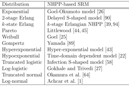
Table 2: Relationship between fault detection time distributions and NHPP-based SRMs
Distribution NHPP-based SRM
Exponential Goel-Okumoto model [26]
2-stage Erlang Delayed S-shaped model [90]
k-state Erlang k-stage Erlangian NHPP [39, 94]
Pareto Littlewood [44, 45]
Weibull Goel [25]
Gompertz Yamada [89]
Hyperexponential Hyper-exponential model [43]
Hypoexponential Time-domain dependent model [22]
Truncated logistic Infection S-shaped model [58]
Log-logistic Gokhale and Trivedi [27]
Truncated normal Okamura et al. [64]
Log-normal Achcar et al. [1]
4.1. NHPP-based SRM
Langberg and Singpurwalla [42] showed that almost all of the NHPP-based SRMs follow a simple debugging scenario, which causes a unified modeling framework for NHPP-based SRMs. Suppose that
(A-1) The total number of software faults is a Poisson random variable with mean ω. (A-2) All of the software fault detection times are IID random variables having a c.d.f.
F (x).
Let M (x) be the cumulative number of software faults before time x. Provided that the total number of software faults is given by N , the number of faults detected before time t follows the binomial distribution with success probability F (x). Then we have
P (M (x) = y|M(∞) = N) = ( N y ) F (x)yF (x)N−y, (4.1)
where F (x) = 1− F (x). Since N is a Poisson random variable with mean ω, the probability mass function (p.m.f.) of M (x) is given by
P (M (x) = y) = ∞ ∑ N =y e−ωω N N ! ( N y ) F (x)yF (x)N−y, = (ωF (x)) y y! e −ωF (x). (4.2)
The above p.m.f. is equivalent to the NHPP with mean value function ωF (x) [42].
Equation (4.2) implies that each of NHPP-based SRMs can be characterized by a par-ticular fault detection time distribution. Table 2 presents relationship between typical fault detection time distributions and corresponding NHPP-based SRMs.
4.2. PH-SRM
Okamura and Dohi [59, 60, 63] proposed PH-SRM (phase-type software reliability model) by substituting the PH distribution to the fault detection time distribution in NHPP-based
model. Then the p.m.f. of M (t) is given by P (M (x) = y) = (ωFP H(x)) y y! e −ωFP H(x), (4.3) FP H(x) = 1− α exp(T x)τ . (4.4)
Since PH distribution can express any distribution approximately, PH-SRM can also express all of the NHPP-based SRMs. Okamura and Dohi [59, 60, 63] considered two specific PH-SRM; CPH-SRM and HEr-SRM that use CF1 and hyper-Erlang distribution, respectively. The fundamental procedure of software reliability assessment with NHPP-based SRMs is (i) to collect the fault data in testing phase, (ii) to estimate model parameters from the collected data, (iii) to compute the reliability measures from the estimated models. Since PH-SRM involves many parameters, we have to say that Step (ii) is not an easy task. Okamura and Dohi [63] developed the EM algorithm for PH-SRM when grouped fault detection data are given.
Let D = {(x1, y1), . . . , (xK, yK)} be grouped data, where yi are the cumulative number of faults in time interval [0, xi). Here we define 0 < X1 < X2 <· · · < XN as all of ordered fault detection times, where N is the number of total faults detected in [0,∞). Note that
Xi and N are unobserved variables. Based on the EM principle, we formulate EM-step of
PH-SRM as follows. ω← E[N|D], (4.5) (α, T , τ )← E [ N ∑ k=1 log fP H(X[k]) ¯¯ ¯¯ ¯ D ] . (4.6)
By applying the result of [69] to Equation (4.5), we have
ω← yK+ ωFP H(xK). (4.7)
On the other hand, Equation (4.6) implies the EM-step for ordinary PH distribution with grouped and truncated data, provided that the total number of faults follows a Poisson distribution. Since N/U is the expected total number of events in Algorithm 2, we obtain the E-step of Equation (4.6) by replacing N/U with ω in Algorithm 2.
In the PH-SRM, the data fitting ability depends on the number of phases. As the number of phases increases, the data fitting ability of PH-SRM also increases. On the other hand, the overfitting problem may arise when the number of phases is excessively large. Information criteria offer plausible measures to prevent the overfitting. The most well-known information criterion is AIC [2], which is defined by
AIC =− 2(maximum log-likelihood) + 2(degrees of freedom), (4.8)
where the degrees-of-freedom is generally identical to the number of free model parameters. The model with the smaller AIC can be regarded as as the better model. Although AIC is quite convenient for the model selection problem, we must carefully treat the definition of degrees-of-freedom. In particular, when dealing with the models involving redundant parameters like mixture models, the degrees-of-freedom is not identical to the number of free parameters. The PH-SRM is the case. It should be noted that there are some open problems to be solved for degrees-of-freedom of PH distribution.
Table 3: Data fitting results
Model MSE MLL DF AIC CTIME
GO 990.20 -359.88 2 723.76 — ISS 295.33 -317.93 3 641.85 — Q-R ISS 230.60 -296.44 5 602.88 — Beta-Mix 278.47 -327.65 2 659.30 — 31-CPH-SRM 44.10 -246.43 23 538.86 1.2 20-HEr-SRM 275.22 -302.10 8 620.20 237.0 4.3. Numerical experiment
We compare PH-SRMs with two NHPP-based SRMs in terms of data fitting ability. Many researchers proposed NHPP-based SRMs under different modeling scenarios. Hwang and Pham [30] proposed an NHPP-based SRM under the scenario that the fault removal is delayed. Based on this scenario, they presented a piecewise continuous mean value function. Kim et al. [40] also discussed a different NHPP-based SRM from the statistical point of view. They incorporated the Beta distribution to represent unknown probability in the model, and unified both finite and infinite failure models. In the above papers, the authors examined the data fitting ability with the exactly same data, and concluded that both models were superior to other well-known SRMs such as Goel-Okumoto model [26], inflection S-shaped model [58], and some others [91], [75], [93]. Here we demonstrate the data fitting ability of our PH-SRM by compared with these latest SRMs under the same data set used in [30, 40]. The data was originally reported by Tohma et al. [83], which consists of 111 observations of the number of detected faults (grouped data) in actual software testing. The tested programs were for the monitoring and real-time control system with about 200 modules, where each module has around 1000 lines of code. Hwang and Pham [30] and Kim et al. [40] derived ML estimates of their SRMs for this data set. The estimated model parameters can be cited in [30, 40].
To evaluate the data fitting ability of our PH-SRM, we estimate model parameters of CPH-SRM and HEr-SRM with the same data. In PH-SRM, we determined the best number of phases from the view point of AIC, and chose 31-CPH-SRM as the best model from 2-CPH-SRM through 50-2-CPH-SRM. On the other hand, the computation time of parameter estimation for HEr-SRM exponentially increases with the number of phases. Thus, in the case of HEr-SRM, we examined AICs for up to 20-HEr-SRM. As a result, 20-HEr-SRM was selected as the best one among them.
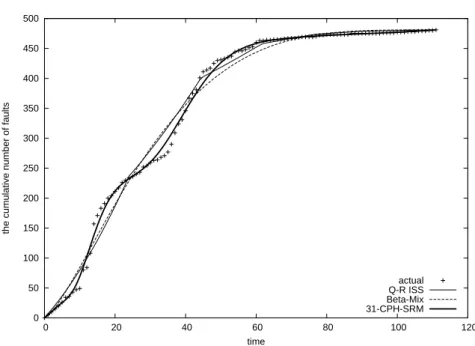
Table 3 presents the summary of fitting results for all the SRMs. GO and ISS denote Goel-Okumoto model [26] and inflection S-shaped model [58], respectively. Q-R ISS means the quasi-renewal time-delay model based on inflection S-shaped mean value function in [30], which was the best model on the original paper [30]. Beta-Mix is an NHPP-based SRM with beta mixture proposed by [40]. Although the above paper just focused on the simplest two mixture models, we chose the best mixture model among others. As the data fitting criteria, we compute mean squared error (MSE), maximum log-likelihood (MLL), degrees of freedom (DF) and AIC‡. Note that the definition of MSE here is also different from [30,40], ‡Note that AIC of Q-R ISS is different from the original paper [30]. The AIC computed in [30] seems to be
0 50 100 150 200 250 300 350 400 450 500 0 20 40 60 80 100 120
the cumulative number of faults
time
actual Q-R ISS Beta-Mix 31-CPH-SRM
Figure 3: The estimated mean value functions
so, for the grouped data {(x1, y1), . . . , (xK, yK)}, MSE is computed by
MSE = 1 K K ∑ k=1 ( ˆ Λ(xk)− yk )2 , (4.9)
where ˆΛ(x) is the estimated mean value function of NHPP-based SRM. The column CTIME
indicates the computation time to obtain ML estimates for 31-CPH-SRM and 20-HEr-SRM. Figure 3 also illustrates the estimated mean value functions for Q-R ISS, Beta-Mix and 31-CPH-SRM. Form the results, 31-CPH-SRM has extremely high data fitting ability compared to others. In fact, although DF of 31-CPH-SRM is higher than others, the mean behavior of 31-CPH-SRM is very close to the actual data in Figure 3. The same observation can be obtained from the result of MSE. This is an evidence that the SRM with high degrees of freedom requires to represent the fault detection processes with many change points on the data trend. Although PH-SRM is built by applying PH distribution to software fault detection time distribution in the framework of Langberg and Singpurwalla [42], PH-SRM is not based on any modeling scenario dissimilar to Q-R ISS, and is superior to the others in terms of data fitting ability. From this simple example, we understand that it is enough to select an appropriate fault detection time distribution in NHPP-based software reliability modeling.
5. PH Approximation for Markov Regenerative Process
Markov modeling is one of the most important techniques to evaluate reliability and perfor-mance of systems. A Markov regenerative process (MRGP) is known as one of the widest class of stochastic counting processes that are mathematically tractable. MRGP consists of several discrete states and time sequence of state transitions, and is an extension of both CTMC and the renewal process. Since MRGP allows state transitions triggered by general distributions, it is often used to analyze stochastic Petri nets. The Markov regenerative stochastic Petri net (MRSPNs), which are governed by MRGP, are heavily used in com-puter science [14, 24, 41]. In this section, we discuss the transient analysis of MRGP by
applying PH approximation. The fundamental idea is to replace general distributions of MRGP with PH distributions that approximate the general distributions. Since the original MRGP is well approximated by a time-homogeneous CTMC, we can derive numerically transient probabilities with commonly-used techniques for CTMC such as uniformization. In particular, this section presents a systematic way to approximate MRGP with a CTMC via PH approximation.
5.1. Markov regenerative process
Consider a stochastic process{S(t); t ≥ 0} with discrete state space. If S(t) has time points at which the process probabilistically restarts itself, the process is called regenerative. When state transitions at the regeneration points are governed by a DTMC, the process S(t) is an MRGP. Define a regeneration time sequence T1 < T2 < · · · and their time intervals
∆Ti = Ti − Ti−1, i = 1, 2, . . .. Then the time intervals can be represented by a Markov renewal sequence [15]. Suppose that the time sequence is time-homogeneous, i.e.,
P (S(Tn) = j, ∆Tn < t | S(Tn−1) = i)
= P (S(T1) = j, ∆T1 < t | S(T0) = i)≡ Ki,j(t). (5.1)
The state probability of MRGP is given by Vi,j(t) = P (S(t) = j | S(0) = i) = P (S(t) = j, ∆T1 ≤ t | S(0) = i) + P (S(t) = j, ∆T1 > t| S(0) = i) =∑ l ∫ t 0 P (S(t− u) = j | S(0) = l)dKi,l(u) + P (S(t) = j, ∆T1 > t| S(0) = i). (5.2)
In general, K(t), V (t) and E(t) are matrices whose elements are given by Ki,j(t), Vi,j(t) and
P (S(t) = j, ∆T1 > t | S(0) = i), respectively. Then we have the Markov renewal equation
for MRGP [14, 21];
V (t) = E(t) + ∫ t
0
dK(u)V (t− u), (5.3)
where E(t) and K(t) are called local and global kernels.
To apply PH approximation, we consider the following MRGP whose space space is finite and each state is classified to subspaces:
• The state space is separated into subspaces SE and SG
1 , . . . ,SKG.
• The subspace SE (EXP state) is a set of the states in which there exist only
exponen-tial (EXP) transitions. C0 is defined as an infinitesimal generator of CTMC for EXP
transitions in the subspace SE. Also C
1, . . . , CK are transition rate matrices for EXP transitions that transfer the state from the subspace SE to the subspaces S1G, . . . ,SKG, respectively.
• The subspace SG
i (GEN states) is a set of the states where there exist both EXP transi-tions and general (GEN) transitransi-tions that are triggered by general distributransi-tions.
– InSG
1 , . . . ,SKG, there is no EXP transition that transfers the state to other subspaces, i.e., all the EXP transitions ofSG
i are the transitions between two states of SiG. Qi denotes the infinitesimal generator of EXP transitions of SiG.
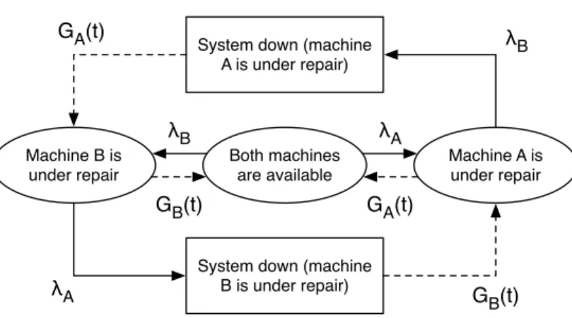
– In SiG, there are Mi GEN transitions that are triggered by general distributions;
G(l)i (t), l = 1, . . . , Mi. These transitions are competitive. That is, when one GEN transition occurs, the ages of the other distributions are renewed.