Vol. 58, No. 4, October 2015, pp. 307–329
MULTI-PERIOD STOCHASTIC PROGRAMMING MODEL FOR STATE-DEPENDENT ASSET ALLOCATION WITH CVAR
Shinya Hirano1 Norio Hibiki
Okasan Asset Management Keio University
(Received February 12, 2014; Revised April 14, 2015)
Abstract We need to solve a multi-period optimization problem to decide dynamic investment policies under various practical constraints. Hibiki (2001,2003,2006) develop a hybrid model where conditional decisions can be made in a simulation approach, and investment proportions are expressed by a step function of the amount of wealth. In this paper, we introduce an idea of a state-dependent function into the hybrid model as well as Takaya and Hibiki (2012). At first, we define the state-dependent function form for a multiple asset allocation problem with CVaR (Conditional Value at Risk) using the hybrid model, and we clarify that the function form is V-shaped and kinked at the VaR point. We propose a piecewise linear model with the V-shaped function to solve the multi-period and state-dependent asset allocation problem. We solve a three-period problem for five assets, and compare the piecewise linear model with the hybrid model. We conduct the sensitivity analysis for different risk averse coefficients and autocorrelations to examine the characteristics of the model.
Keywords: finance, stochastic optimization, multi-period asset allocation, simulation
1. Introduction
Institutional investors need to manage their investment funds in consideration of rebalanc-ing assets durrebalanc-ing a plannrebalanc-ing period for efficient asset management. Individual investors who face their long-term financial planning have similar problems. A multi-period optimization model involving dynamic investment decisions explicitly can be used to solve the problem with several constraints in practice. There are many studies in the literatures of different academic fields. In the fields of mathematical finance and financial economics, analytical so-lutions or approximate soso-lutions are derived employing the HJB equation or the Martingale method under the setting of a continuous time and a continuous distribution. Cvitani´c and Karatzas [3] derive a closed form solution of minimizing the first-order lower partial moment (LPM).2 Recently, several Monte Carlo methods have been developed for the computation
of optimal portfolio policies (Detemple, Garcia and Rindisbacher [4]). But the number of assets is limited to solve the problem in general, and it is also difficult to derive the optimal solutions for the model with practical constraints. In the fields of financial engineering, the numerical solutions are derived employing mathematical programming under the setting of a discrete time and a discrete distribution in order to solve the multiple assets problem with practical constraints. Hibiki [5] develops a simulated path model to solve the multi-period portfolio optimization problem. A return distribution is described using simulated paths
1This research is done in the Graduate School of Science and Technology, Keio University. The research
achievement is not associated with Okasan Asset Management Co., Ltd.
2Siegmann [11] shows that an optimal investment policy is V-shaped in terms of wealth in the case of
maximizing the objective function, which is the expected wealth minus the second-order lower partial moment in a discrete time and a binomial distribution.
generated by the Monte Carlo method. Hibiki [6, 8, 9] develop a hybrid model involving conditional decisions in the simulated path approach.3 In the hybrid model, similar states are bundled at each time so that the same conditional decisions can be made, though the decisions are not strictly state-dependent.
The solution methods of these two approaches are different from each other. When the optimization problem is solved analytically, the analytical solution is expressed as the state-dependent function. When the mathematical programming problem is solved, the optimal solutions are derived numerically. There does not exist an integrated model of these approaches except Takaya and Hibiki [13] which propose a linear approximation model to derive a state-dependent asset allocation in a discrete time and a discrete distribution and solve a two-asset problem with a risky asset and a riskless asset to compare it with the analytical solutions.
The purpose of this paper is to introduce the idea of the state-dependent function into the hybrid model as well as Takaya and Hibiki [13], and to construct the integrated model of both stochastic programming approach and analytical approach for multiple assets problem. Specifically, we propose the multi-period optimization model involving state-dependent de-cision making with the conditional value at risk (CVaR) [10], rather than the lower partial moment as a risk measure. CVaR is a well-known risk measure defined as the expected loss based on a given loss tolerance.
The contributions and characteristics of our paper involving the comparison with the previous studies are in what follows.
(1) Definition of the state-dependent function for CVaR
Using the hybrid model, we define the state-dependent function form for the problem where the objective function is the expected terminal wealth minus the CVaR of the terminal wealth. We clarify that the function form is V-shaped and kinked at VaR in the case of the CVaR risk measure.4 However, our conclusion is numerically drawn,
but cannot be proved theoretically. We conduct the analysis for a three-asset problem including two risky assets and a riskless asset where two risky assets are correlated and autocorrelated with each other, and draw the conclusion. Moreover, we discuss the characteristics of a piecewise linear (’PwL’ hereafter) model through the analysis for a five-asset problem.
(2) Overcoming a drawback of the hybrid model with respect to the optimal weights The optimal weights are assumed to be expressed as a step function of the amount of wealth in the hybrid model because they are derived discretely for the decision nodes. Therefore, there is the drawback that the optimal weights may change significantly even if the amount of wealth is changed only slightly because the states belonging in the decision nodes lying next to each other may have similar amounts of wealth from each other. We can overcome the drawback by employing the state-dependent and continuous function.
3A scenario tree model is widely used in a mathematical programming approach (Ziemba and Mulvey [16],
Zenios and Ziemba [14, 15]). However, the numbers of decision variables and constraints in the scenario tree may grow exponentially to ensure that the constructed representative set of scenarios covers the set of possibilities to a sufficient degree.
4Takano and Gotoh [12] solve the optimization model with CVaR in the simulated path approach as well
as our paper, and a nonlinear control policy is derived using the kernel method. However, it is difficult to advice the investment action in practice because the weights derived discretely cannot be expressed explicitly by the state-dependent function. In this paper, it is possible to express the investment weights by the state-dependent function with respect to the amount of wealth in a real world.
(3) Consistent results with other risk measures
In the minimization problem of the first-order lower partial moments of wealth, Cvitani´c and Karatzas [3] show that the optimal weight of a risky asset is zero if the amount of wealth is larger than a discounted value of the target wealth, and otherwise the optimal weight is expressed by a nonlinear function of wealth. In the same manner, Siegmann [11] shows that an optimal investment policy is V-shaped in terms of wealth in the case that the objective function is the expected wealth minus the second-order lower partial moment multiplied by risk aversion. The optimal policy is V-shaped and state-dependent in terms of wealth, and kinked at the target wealth associated with the risk measure. The function form derived using the linear approximation model of our paper is consistent with that of the previous models.
(4) Developing the PwL model with a state-dependent function for a more than three-asset problem
We develop the PwL model for a N -asset problem involving the state-dependent investment unit function, and compare it with the hybrid model. We conduct the numerical analysis for a five-asset optimization problem and examine the usefulness of the model.
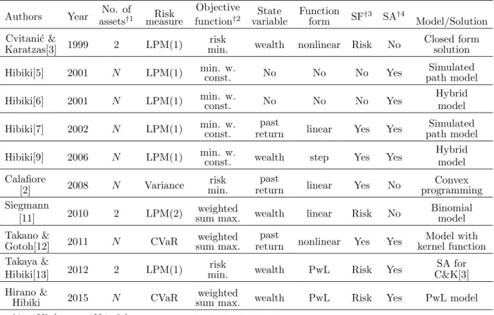
Table 1: Comparison of our paper with the previous studies
Authors Year assetsNo. of†1 measureRisk functionObjective†2 variableState Functionform SF†3 SA†4 Model/Solution Cvitani´c &
Karatzas[3] 1999 2 LPM(1)
risk
min. wealth nonlinear Risk No
Closed form solution Hibiki[5] 2001 N LPM(1) min. w.const. No No No Yes path modelSimulated
Hibiki[6] 2001 N LPM(1) min. w.const. No No No Yes Hybridmodel
Hibiki[7] 2002 N LPM(1) min. w.const. returnpast linear Yes Yes path modelSimulated
Hibiki[9] 2006 N LPM(1) min. w.const. wealth step Yes Yes Hybridmodel Calafiore
[2] 2008 N Variance
risk min.
past
return linear Yes No
Convex programming Siegmann
[11] 2010 2 LPM(2)
weighted
sum max. wealth linear Risk No
Binomial model Takano & Gotoh[12] 2011 N CVaR weighted sum max. past
return nonlinear Yes Yes
Model with kernel function Takaya &
Hibiki[13] 2012 2 LPM(1)
risk
min. wealth PwL Risk Yes
SA for C&K[3] Hirano &
Hibiki 2015 N CVaR
weighted
sum max. wealth PwL Risk Yes PwL model
†1 ‘N’ denotes ‘N ≥ 3 ’
†2 ‘min. w. const.’ denotes ‘minimization with constraints’
†3 State-dependent Function (If a weight function is a state-dependent function, then ‘Yes’.
If the SF form is determined based on a risk measure, then ‘Risk’.)
We show Table 1 to compare our paper with the previous studies of the simulated path approach5 and their referred studies, and clarify the differences.
This paper is organized as follows. In Section 2, we clarify the relationship between wealth and investment weights using the hybrid model. In Section 3, we propose the op-timization model with a PwL function which is state-dependent in terms of wealth for the CVaR problem. In Section 4, we solve a five-asset and three-period problem. The PwL model is compared with the hybrid model, and the usefulness of the model is examined. In addition, we conduct the sensitivity analysis for two kinds of parameters; risk aversion and autocorrelation. Section 5 provides our concluding remarks.
2. Modeling using state-dependent function with CVaR
2.1. Hybrid model and conditional decision
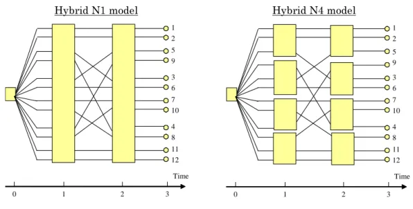
The hybrid model allows conditional decisions to be made for similar states bundled at each time using sample returns generated by the Monte Carlo method [6, 8, 9]. We can use a tree or lattice structure to make conditional decisions.6 A rule that the same investment decisions are made in similar states is defined to satisfy the non-anticipativity.
1 2 3 0 Time 5 9 1 2 3 6 7 10 4 8 11 12 1 2 3 0 Time 5 9 1 2 3 6 7 10 4 8 11 12 Hybrid N4 model Hybrid N1 model
Figure 1: Hybrid model structures
We employ the lattice structure as the modeling structure with respect to the decision nodes in this paper. We call ‘hybrid Nm model’ for the hybrid model with m decision nodes at each time hereafter. A decision node is defined as a set of states at each time, and a path is defined as a set of states through time. As examples of the lattice structure, we depict the hybrid N1 model 7 on the left-hand side of Figure 1 and the hybrid N4 model on the right-hand side, respectively. The number of paths is twelve and the same decision is made for paths in each node at each time.
Hibiki [7] proposes an investment unit function to express the decision rule which is defined to satisfy the non-anticipativity condition in the simulated path model. Hibiki [8, 9]
5The simulated path approach is proposed by Hibiki [5, 6] where sample paths are generated using the
Monte Carlo method and the optimal solutions are derived in the multi-period optimization model. The simulated path model [5] and the hybrid model [6] are the basic models.
6Bogentoft, Romeijn and Uryasev [1] solve an ALM problem for pension funds using the hybrid model with
a lattice structure by reference to Hibiki [6].
also propose the investment unit function in the hybrid model to describe the decision rule in the similar states. The investment unit function is defined as Equation (2.1) and we describe the path-dependent investment unit for path i using the base investment decision variable zs
jt for asset j, time t and decision node s.
h(i)(zjts) = a(i)jtzjts (2.1)
where a(i)jt is the investment unit parameter which depends on the decision rule or the investment strategy. There are various ways to decide the parameter values of a(i)jt, and we show two investment strategies as follows.8
(1) Fixed-unit strategy: a(i)jt = 1, or zjts denotes the investment unit (2) Fixed-proportion strategy: a(i)jt = W
(i)
t
ρ(i)jt , or z s
jt denotes the investment proportion, where
ρ(i)jt is a price of risky asset j of path i at time t and Wt(i) is the amount of wealth of path i at time t
We can simply describe the hybrid models involving various decision rules by employing the investment unit functions.
In this paper, we use the hybrid model involving the lattice structure to decide the investment with the state-dependent step function. When we have I states and m nodes at each time, we have (about) mI states in each node. We sort the states by the amount of wealth at each time.
2.2. Formulation of the hybrid model
We formulate the hybrid model for the asset allocation problem. A terminal loss with respect to the amount of wealth is defined as a negative deviation from the amount of initial wealth, and both VaR and CVaR of the loss distribution are calculated.
The objective function is expressed by the expected terminal wealth minus CVaR mul-tiplied by a constant γ. Notations used in the formulation are as below.
(1) Notations
1
⃝ Sets
St: set of fixed-decision nodes s at time t, (t = 1, . . . , T − 1)
Vts−1: set of paths passing any node s at time t− 1, (t = 2, . . . , T ; s ∈ St−1) 2
⃝ Parameters
n : number of risky assets T : number of periods I : number of sample paths
ρj0: price of risky asset j at time 0, (j = 1, . . . , n)
ρ(i)jt : price of risky asset j of path i at time t, (j = 1, . . . , n; t = 1, . . . , T ; i = 1, . . . , I)
r0: interest rate in period 1
r(i)t−1: interest rate in period t (the rate of path i at time t− 1 is used), (t = 2, . . . , T ; i = 1, . . . , I)
W0: initial amount of wealth.
8Hibiki [7] formulates the models with the investment unit functions which show a trend following strategy,
a contrarian strategy, and a strategy using autocorrelation. The investment unit function is expressed as a linear function of the previous rate of return.
γ : risk aversion
3
⃝ Variables
zj0: investment unit for asset j and time 0, (j = 1, . . . , n)
zjts : base investment variable for asset j, time t, and node s (j = 1, . . . , n; t = 1, . . . , T − 1; s ∈ St−1)
Wt(i): amount of wealth of path i at time t, (t = 1, . . . , T ; i = 1, . . . , I) VaR : VaR at a β confidence level 9
CVaR : CVaR at a β confidence level
q(i): deviation of the loss above VaR, (i = 1, . . . , I)
(2) Formulation
The hybrid Nm model is formulated as follows.
Maximize 1 I I ∑ i=1 WT(i)− γ · CVaR (2.2) subject to n ∑ j=1 ρj0zj0 = W0 (2.3) W1(i) = n ∑ j=1 ρ(i)j1zj0 (i = 1, . . . , I) (2.4) Wt(i) = n ∑ j=1 { ρ(i)jt − ( 1 + r(i)t−1 ) ρ(i)j,t−1 } h(i)(zj,ts −1) + ( 1 + r(i)t−1 ) Wt(i)−1 (t = 2, . . . , T ; s∈ St−1; i∈ Vts−1) (2.5)
WT(i)+ VaR + q(i) ≥ W0 (i = 1, . . . , I) (2.6)
CVaR = VaR + 1 (1− β)I I ∑ i=1 q(i) (2.7) h(i)(zj,ts −1) = ( Wt(i)−1 ρ(i)j,t−1 ) zj,ts −1, (j = 1, . . . , n; t = 2, . . . , T ; s∈ St−1; i∈ Vts−1) (2.8) zj0 ≥ 0 (j = 1, . . . , n) (2.9) zjts ≥ 0 (j = 1, . . . , n; t = 1, . . . , T − 1; s ∈ St) (2.10) q(i) ≥ 0 (i = 1, . . . , I) (2.11)
Equation (2.3) is a budget constraint which shows the full investment in risky assets. Equa-tion (2.5) is the calculaEqua-tion of the amount of wealth at time t derived by the investment at time t− 1. Equations (2.6) and (2.7) are used to calculate CVaR.
The optimal weights are derived numerically at each discrete decision node including a set of states in the hybrid Nm model with the fixed-proportion strategy, and therefore they are not strictly state-dependent.10 We examine the relationship between amounts of
9The values of VaR and CVaR are dependent on β. However we omit β in the expressions to avoid complicate
presentation.
wealth and investment weights using the hybrid N25 model in order to introduce an idea of a state-dependent function derived in the analytical approach into the hybrid model in the next section.
2.3. Numerical analysis using the hybrid model
The relationship is examined using the hybrid model with three assets, three periods and 25 nodes in order to approximate the state-dependent function. Details of the numerical analysis are as follows.
• Three assets consist of two risky assets and a riskless asset.
— The rates of return of risky assets are normally distributed. The relationship is investigated using the parameters of three kinds of correlations between two risky assets (ρ = −0.5, 0, 0.5) and three kinds of autocorrelations (c = −0.5, 0, 0.5). The following correlation matrices are supposed, where Ai(t) denotes asset i at time t.
Correlation Cross-correlation (lag 1) Cross-correlation (lag 2)
A1(t) A2(t) A1(t) A2(t) A1(t) A2(t)
A1(t) 1 ρ A1(t + 1) c ρc A1(t + 2) 0.5c 0.5ρc
A2(t) ρ 1 A2(t + 1) ρc c A2(t + 2) 0.5ρc 0.5c
— Both the expected value and standard deviation of the rate of return of risky asset 1 are larger than those of risky asset 2. (r1 = 5%, σ1 = 20%; r2 = 2%, σ2 = 5%)
— The risk-free rate is 0%.
• The initial amount of wealth is 100 million yen.
• The CVaR is calculated at a 80% confidence level with 50,000 sample paths.
• The problem is solved using the iterative algorithm developed by Hibiki [9]. We utilize the
hybrid N1 model with the fixed-unit strategy in the first step, and the fixed-proportion strategy in the second step. We utilize the hybrid N25 model with the fixed-proportion strategy in the subsequent steps until the objective function value converges. In the hybrid N25 model, the lattice structure is generated by sorting the amounts of wealth calculated after each iteration, and dividing them into 25 sets. The number of states in a decision node is 2,000 because of 50,000 paths and 25 nodes.
• Two cases are analyzed as follows.
(Case 1) Optimization problems are solved for three kinds of risk averse coefficients under the conditions that (1a) no cash borrowing is allowed, and (1b) cash borrowing which limit ratio is 100% is allowed. No correlation and no autocor-relation (ρ = 0, c = 0) are supposed in these cases.
(Case 2) CVaR minimization problems are solved for the combination of three kinds of correlations and three kinds of autocorrelations under the condition that cash borrowing is allowed.
2.3.1. Case 1a
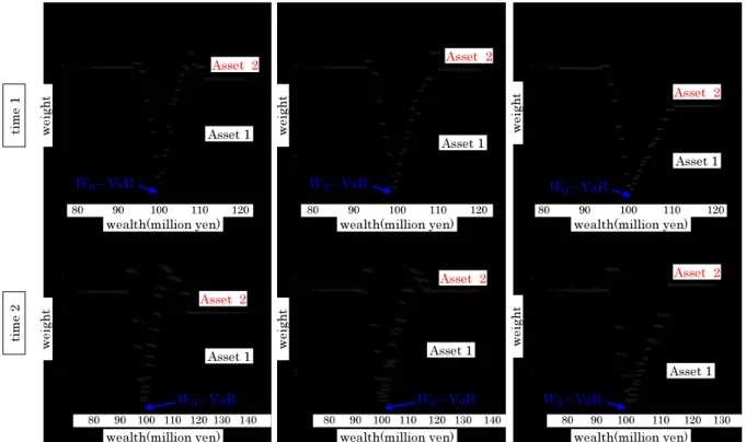
We show the scatter plot of amounts of wealth vs. investment weights to examine the relationship between them in Figure 2. The optimal weights are almost V-shaped with respect to the amounts of wealth.11 Specifically, the weights of risky assets are the smallest
It is not constrained that the optimal weight function is stepwise explicitly in the formulation, but it is expected because decision nodes are generated discretely by employing sorted amounts of wealth.
11The optimal weights may not look V-shaped for the small or large amounts of wealth. This reason is that
ç= 2 ç= 4 ç! 1(Risk minimization)
wealth(million yen)
Asset 2
Asset 1
W0
ÄVaR W0ÄVaR W0ÄVaR
W0ÄVaR W0ÄVaR W0ÄVaR w e ig h t w e igh t w e igh t w e igh t w e igh t w e ig h t Asset 2 Asset 2 Asset 1 Asset 1 Asset 1 Asset 1 Asset 1 Asset 2 Asset 2 Asset 2
wealth(million yen) wealth(million yen)
wealth(million yen) wealth(million yen) wealth(million yen)
80 90 100 110 120 80 90 100 110 120 80 90 100 110 120 80 90 100 110 120 130 140 80 90 100 110 120 130 140 80 90 100 110 120 130 tim e 1 tim e 2
Figure 2: Relationship between amounts of wealth and investment weights for no correlation and no autocorrelation case (of ρ = 0, c = 0, Case 1a). Each point shows each sample value.
at the VaR point of wealth, W0−VaR, which is the initial wealth minus the value at risk
of terminal wealth. The optimal weight tends to increase as the amount of wealth moves away from the VaR point. These results are consistent with Cvitani´c and Karatzas [3] and Siegmann [11] which show that optimal investment policies are kinked at a target wealth, and piecewise or V-shaped in terms of wealth under the lower partial moment (LPM).12 The target levels are different between the CVaR and the LPM, however they are used in calculating downside risk measures. It is reasonable the optimal weights are kinked at the VaR point as well as the LPM because the VaR is a target wealth when calculating the CVaR.
We have a different point between the CVaR and the LPM with respect to the function form for the risk minimization problem. While the optimal weights of risky assets are zero above the discounted target wealth for the LPM minimization problem, they are not zero even above the target (W0−VaR) for CVaR minimization problem. This reason is that the
amounts of terminal wealth and its VaR can be controlled and the CVaR can be improved by investing risky assets during a planning period.
The weight function of asset 1 with larger expected return and volatility is clearly V-shaped in terms of wealth. On the other hand, the weight of asset 2 is also V-V-shaped
large amounts of wealth, respectively.
12The first-order LPM is minimized in Cvitani´c and Karatzas [3], and a discounted target wealth is the
kinked point of the piecewise function. On the other hand, the expected asset values minus the second-order LPM multiplied by the risk aversion is maximized in Siegmann [11], and a target asset value minus a certain value is a kinked point of V-shaped function. It is expected that the location of the kink is a discounted wealth of W0−VaR when minimizing CVaR, and therefore the modification of W0−VaR should be applied
strictly. But we employ W0−VaR as the kinked point because it is difficult to find the point. The method
around the VaR point, but it does not keep its shape in larger and smaller amounts of wealth because of the non-negative constraint of cash. Next, we solve the problem without the non-negative constraint of cash to examine the reason.
2.3.2. Case 1b
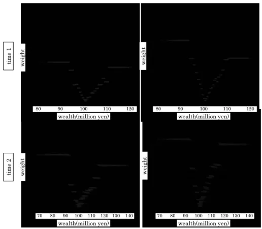
The weights of risky assets are subject to the cash borrowing constraint because the upper bound of the sum of the weights is one in the Case 1a where no cash borrowing is allowed. We compare two cases between cash borrowing allowed and no cash borrowing allowed to examine the effect of the cash borrowing constraint. We show the results for γ = 4 in Figure 3. The results of no cash borrowing case are the same as Figure 2.
w e ig h t w e igh t ti me 1 ti me 2 Asset 1 wealth(million yen) 80 90 100 110 120 Asset 2 wealth(million yen) 70 80 90 100 110 120 130 140 w e igh t wealth(million yen) 80 90 100 110 120 w e ig h t wealth(million yen) 70 80 90 100 110 120 130 140
Cash borrowing allowed
No cash borrowing Cash borrowing allowed
No cash borrowing
Cash borrowing allowed
No cash borrowing Cash borrowing allowed
No cash borrowing w e ig h t w e igh t ti me 1 ti me 2 Asset 1 wealth(million yen) 80 90 100 110 120 Asset 2 wealth(million yen) 70 80 90 100 110 120 130 140 w e igh t wealth(million yen) 80 90 100 110 120 w e ig h t wealth(million yen) 70 80 90 100 110 120 130 140
Cash borrowing allowed
No cash borrowing Cash borrowing allowed
No cash borrowing
Cash borrowing allowed
No cash borrowing Cash borrowing allowed
No cash borrowing
Figure 3: Comparison between two cases: Case 1a vs Case 1b
We notice that the points in the plots of two cases are not overlapped even if the sum of the weights are below one because the value of W0−VaR∗ in the cash borrowing case is
larger than the value in the no cash borrowing case. We find that the weight of asset 2 can be also V-shaped in large and small amounts of wealth with cash borrowing allowed. This shows that the weights are subject to the upper bound for small and large amounts of wealth in Case 1a.
2.3.3. Case 2
We also examine the relationship for the combination of three kinds of correlations and three kinds of autocorrelations under the CVaR minimization. We show the results at time 1 in Figure 4.
We find different shapes at each graph. For c = 0, we find a set of points is typically V-shaped. We note the weight of asset 1 is smaller than the weight of asset 2 because the volatility of asset 1 is larger than that of asset 2. For c = −0.5, the weight of asset 1 is small above the VaR point. The reason is as follows. We get the large amount of wealth
at time 1 when a positive return is generated in period 1. But a positive return at time 1 for c =−0.5 is likely to be a negative return at time 2 because asset returns are negatively autocorrelated. Therefore the weight of asset 1 is not likely to be invested above the VaR point. In a similar manner, the weight of asset 1 is small below the VaR point for c = 0.5.
Even if there are no slopes above and below the VaR point, we can also formulate the model with the state-dependent functions which are V-shaped and kinked at the VaR as well as in Case 1. 2 50 2 00 1 50 1 00 5 0 0 8 00 0 9 00 0 1 00 0 0 1 10 0 0 1 20 0 0 1 30 0 0 1 50 1 00 5 0 0 7 00 0 8 00 0 9 00 0 1 00 0 0 1 10 0 0 1 20 0 0 1 30 0 0 2 00 1 50 1 00 5 0 0 7 00 0 8 00 0 9 00 0 1 00 0 0 1 10 0 0 1 20 0 0 1 30 0 0 2 00 1 50 1 00 5 0 0 9 00 0 9 50 0 1 00 0 0 1 05 0 0 1 10 0 0 1 15 0 0 1 40 1 20 1 00 8 0 6 0 4 0 2 0 0 8 00 0 9 00 0 1 00 0 0 1 10 0 0 1 20 0 0 1 20 1 00 8 0 6 0 4 0 2 0 0 8 00 0 9 00 0 1 00 0 0 1 10 0 0 1 20 0 0 2 00 1 50 1 00 5 0 0 9 00 0 9 50 0 1 00 0 0 1 05 0 0 1 10 0 0 1 15 0 0 1 20 0 0 1 50 1 00 5 0 0 8 00 0 9 00 0 1 00 0 0 1 10 0 0 1 20 0 0 6 0 5 0 4 0 3 0 2 0 1 0 0 9 00 0 1 00 0 0 1 10 0 0 1 20 0 0 Correlation Auto correlation 0 0. 5 1. 0 1. 5 2. 0 2. 5
W0ÄVaR W0ÄVaR Asset 1 W0ÄVaR
Asset 2 Asset 2 Asset 1 c=Ä0:5 c= 0 c= 0:5 ö= Ä0:5 ö= 0 ö= 0:5 w e ig h t wealth(million yen) 80 90 100 110 120 130 wealth(million yen) 70 80 90 100 110 120 130 0 0. 5 1 .0 1. 5 w e ig h t wealth(million yen) 70 80 90 100 110 120 130 Asset 1 Asset 2 0 0. 5 1 .0 1. 5 2. 0 w e ig h t 0 0. 5 1 .0 1. 5 2. 0 w e ig h t 0 0. 2 0 .4 0 .6 0 .8 1 .0 1. 2 1. 4 w e ig h t 0 0. 2 0 .4 0. 6 0 .8 1. 0 1. 2 w e ig h t 0 0. 5 1 .0 1. 5 2. 0 w e ig h t 0 0. 5 1 .0 1. 5 w e ig h t 0 0. 1 0 .2 0. 3 0 .4 0. 5 0 .6 w e ig h t wealth(million yen) 80 90 100 110 120 wealth(million yen) 90 95 100 105 110 115 wealth(million yen) 80 90 100 110 120 wealth(million yen) 80 90 100 110 120 wealth(million yen) 90 95 100 105 110 115 120 wealth(million yen) 90 100 110 120 Asset 2 Asset 1 Asset 1 Asset 2 Asset 2 Asset 1 Asset 2 Asset 1 Asset 2 Asset 1 Asset 1 Asset 2
Figure 4: Comparison between different correlations and autocorrelations at time 1 under CVaR minimization (Case 2)
2.3.4. Sensitivity of the weight to the amount of wealth
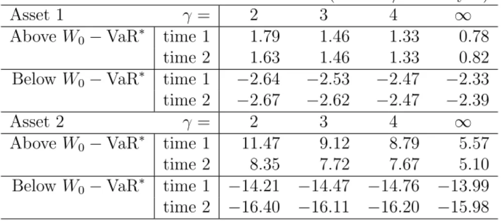
We find the slopes of the function are different between above and below W0−VaR. They
show the sensitivities of the weights to the amount of wealth, as follows, Sensitivity = Change in weight (%) from the weight of ‘W0−VaR’
Change in wealth (million yen) from ‘W0−VaR’
. (2.12)
We can derive the sensitivity using regression. We show the sensitivity of the weight in Table 2 for the different risk averse coefficients of Case 1a. The absolute sensitivity below W0−VaR
is larger than the sensitivity above W0−VaR because we need to increase the amount of
wealth in order to take risk by increasing the weights of risky assets. The absolute sensitivity becomes small to avoid taking risk as the risk averse coefficient (γ) becomes large.
Table 2: Sensitivity of the weight to the amount of wealth (unit: %/million yen)
Asset 1 γ = 2 3 4 ∞
Above W0− VaR∗ time 1 1.79 1.46 1.33 0.78
time 2 1.63 1.46 1.33 0.82
Below W0− VaR∗ time 1 −2.64 −2.53 −2.47 −2.33
time 2 −2.67 −2.62 −2.47 −2.39
Asset 2 γ = 2 3 4 ∞
Above W0− VaR∗ time 1 11.47 9.12 8.79 5.57
time 2 8.35 7.72 7.67 5.10
Below W0− VaR∗ time 1 −14.21 −14.47 −14.76 −13.99
time 2 −16.40 −16.11 −16.20 −15.98
2.3.5. Findings
These results show the two useful findings below.
• It is useful to employ the hybrid model in order to find the state-dependent function
form in the simulated path approach.
• The state-dependent function form is affected by the critical value to evaluate the risk
measure such as the target wealth for LPM and the VaR point for CVaR.
3. Piecewise Linear Model
3.1. Developing the investment unit function with CVaR
We adopt a PwL function form to represent a state-dependent behavior because the weights are nearly proportional to the amount of wealth in Figures 2 to 4, and the large scale problem can be solved in the simulated path approach. However, the sum of the weights for risky assets needs to be subject to the cash constraints in the largest and smallest amounts of wealth and the non-negativity constraints. Therefore, we propose the investment unit function in Equation (3.1) with the investment weight(wjt(i)) which is the PwL function of the amount of wealth at each time(Wt(i)) in Equation (3.2). We call the model with the following functions the PwL model.
h(i)(wjt(i)) = ( Wt(i) ρ(i)jt ) w(i)jt (j = 1, . . . , n; t = 1, . . . , T − 1; i = 1, . . . , I), (3.1) wjt(i) = a1jt+ b1jtθjt1 (Wt(i) ≤ θjt1)
a1jt+ b1jtWt(i) (θjt1 < Wt(i) ≤ W0 − VaR)
a2jt+ b2jtWt(i) (W0− VaR < Wt(i) ≤ θ2jt)
a2 jt+ b2jtθjt2 (W (i) t > θ2jt) , (j = 1, . . . , n; t = 1, . . . , T − 1; i = 1, . . . , I) (3.2) vjt = a1jt+ b 1 jt(W0− VaR) = a2jt+ b 2 jt(W0− VaR), (j = 1, . . . , n; t = 1, . . . , T − 1) (3.3) where a1
jt and a2jt are the intercept coefficients, b1j,t and b2j,t are the slope coefficients, θjt1 and θjt2 are the boundaries of the amount of wealth where the weight of risky asset j
be-comes constant as shown in Figure 5. Specifically, θ1
jt and θ2jt are determined, subject to n
∑ j=1
wjt(i) ≤ 1 − LC and w(i)jt ≥ 0, where LC is a lower bound of cash.
Figure 5: PwL function with no cash borrowing allowed
Equation (3.3) is the constraint which imposes the condition that the weights of two linear functions coincide with each other at the point of W0−VaR. We need to utilize the
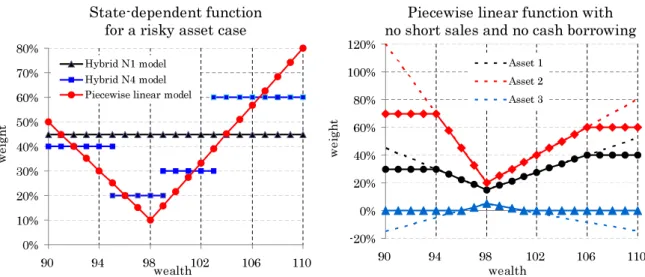
iterative algorithm to solve the problem as well as the hybrid model. Details are explained in Section 3.3. We show the examples of the relationship between wealth and investment weights for the PwL model and the hybrid model on the left-hand side of Figure 6.
Piecewise linear function with no short sales and no cash borrowing State-dependent function
for a risky asset case
-20% 0% 20% 40% 60% 80% 100% 120% 90 94 98 102 106 110 wealth w ei gh t Asset 1 Asset 2 Asset 3 0% 10% 20% 30% 40% 50% 60% 70% 80% 90 94 98wealth102 106 110 w ei gh t Hybrid N1 model Hybrid N4 model Piecewise linear model
Figure 6: State-dependent decision (Relationship between wealth and weight) The state-dependent function of the proposed model is continuous and V-shaped, while that of the hybrid model is discrete and stepwise. The investment decision for the hybrid model with a small number of nodes may be dependent on a method of separating decision nodes. On the other hand, the PwL model with a small number of decision variables is expected to have the same structure as the hybrid model with a lot of decision variables. The both discrete and continuous functions are expected to be similar to each other as on the left of Figure 6. In addition, the investment proportions may change drastically in the hybrid model even if the states belonging in the decision nodes lying next to each other do not have different amounts of wealth. This can be resolved by using the PwL model.
Next, we show an example of the PwL functions for three risky assets on the right of Figure 6. The dotted lines show the functions with short sales for risky assets and cash borrowing allowed, and the solid lines with data markers show the functions without short sales and cash borrowing allowed.13
The PwL model is one of the variations of the hybrid model with two decision nodes where the partition boundary of two nodes is W0−VaR. We can apply the formulation of
the hybrid model in Section 2.2 into the PwL model with some modifications.
3.2. Formulation
We formulate the PwL model based on the hybrid model. We also use the sets, the param-eters and the variables defined in Section 2.2. In this section, we introduce other decision variables as follows, instead of decision variables zs
jt for the hybrid model.14 We use different decision variables for each model. In order to clarify it, we attach ‘[Unit (N1)]’ to the hybrid N1 model with the fixed-unit strategy, ‘[Proportion (N1)]’ to the hybrid N1 model with the fixed-proportion strategy, and ‘[PwL]’ to the PwL model.
(1) Decision variables
wjt: [Unit (N1)] investment unit for asset j and time t (j = 1, . . . , n; t = 1, . . . , T − 1) [Proportion (N1)] investment proportion for asset j and time t
(j = 1, . . . , n; t = 1, . . . , T − 1)
wjt(i): [PwL] investment proportion for asset j, time t and path i (j = 1, . . . , n; t = 1, . . . , T − 1; i = 1, . . . , I)
aujt, bujt: [PwL] intercept and slope of the PwL function of the investment
proportion for asset j and time t (u = 1, 2; j = 1, . . . , n; t = 1, . . . , T − 1)
(2) Formulation
We can formulate the PwL model by modifying the formulation of the hybrid model in Section 2.2. The constraints (3.1) to (3.3) are added to the formulation. In addition, we replace the constraint (2.5) with the following constraint (3.4), and (2.10) with (3.5), respectively. Wt(i) = n ∑ j=1 { ρ(i)jt − ( 1 + r(i)t−1 ) ρ(i)j,t−1 } h(i)(w(i)j,t−1) + ( 1 + rt(i)−1 ) Wt(i)−1 (t = 2, . . . , T ; i = 1, . . . , I) (3.4) w(i)jt ≥ 0, (j = 1, . . . , n; t = 1, . . . , T − 1; i = 1, . . . , I), (3.5)
3.3. Iterative algorithm for the PwL model
The weights of the risky assets are expressed by the state-dependent and PwL function of the amount of wealth as in Equation (3.2). However, it is difficult to solve the problem because it is formulated with the non-linear and non-convex function, and the PwL function is divided at the VaR point and two boundaries (θ1
jt and θ2jt), determined by the amount of wealth. Therefore, we solve the problem using the modification of iterative algorithm developed by Hibiki [9].
If the amounts of wealth, VaR and two boundaries are parameters in Equation (3.1) and (3.2), the original problem can be reduced to a LP problem. Then we replace the values
13Strictly, the dotted lines are expected to be located slightly on the right side of the solid lines as in Figure
3 because of no constraints.
14The investment unit for asset j and time 0 is also denoted by z
derived in the previous iteration into the unknown variables, and solve the LP problem iteratively. The algorithm has the following six steps.
Step 1: We set up h(i)(w
jt) = wjt as the investment unit function. We solve a problem using the hybrid N1 model with the fixed-unit strategy.15 Let Obj0 denote the objective
function value, and set k = 1.
Step 2: Let Wt(k(i)∗−1) be the amount of wealth of path i at time t, and we calculate it. We
set up h(i)(wjt) = (
Wt(k(i)∗−1)
ρ(i)jt
)
wjt as the investment unit function at the k-th iteration, and solve the problem using the hybrid N1 model with the fixed-proportion strategy. We calculate the objective function value Objk.
Step 3: Go to Step 4 if a value Objk − Objk−1 is lower than a tolerance. Otherwise, set
k ← k + 1, and return to Step 2.
Step 4: Set k ← k + 1. Wt(k(i)∗−1) and VaR∗k−1 are calculated as the amount of wealth of
path i at time t and VaR of the (k− 1)th iteration, respectively. We solve the problem using Equations (3.8)-(3.10) instead of Equations (3.1)-(3.3), with short sales allowed and without the cash constraint.
h(i)(w(i)jt) = ( Wt(k(i)∗−1) ρ(i)jt ) wjt(i) (t = 1, . . . , T − 1), (3.8) w(i)jt = { a1 jt+ b1jtW (i)∗ t(k−1) (W (i)∗ t(k−1) ≤ W0 − VaR∗k−1) a2 jt+ b2jtW (i)∗ t(k−1) (W (i)∗ t(k−1) > W0− VaR∗k−1) , (3.9) a1jt + b1jt(W0− VaR∗k−1) = a2jt+ b 2 jt(W0− VaR∗k−1). (3.10)
Step 5: Set k ← k + 1. Wt(k(i)−1)∗ , VaR∗k−1, θ1∗
j,t(k−1) and θ 2∗ j,t(k−1) are calculated as W (i) t , VaR, θ1
jt and θ2jt of the (k− 1)th iteration, respectively. Specifically, θ1j,t(k∗ −1) and θ
2∗
j,t(k−1)
are determined as the boundaries of the amounts of wealth, using Wt(k(i)∗−1), au∗
j,t(k−1) and
bu∗
j,t(k−1)(u = 1, 2). We solve the problem using Equations (3.8), (3.10), and (3.11).
wjt(i) = a1 jt+ b1jtθ1j,t(k∗ −1) (W (i)∗ t(k−1)≤ θ 1∗ j,t(k−1))
a1jt+ b1jtWt(k−1)(i)∗ (θj,t(k1∗ −1) ≤ Wt(k−1)(i)∗ ≤ W0− VaR∗k−1)
a2 jt+ b2jtW (i)∗ t(k−1) (W0− VaR∗k−1 < W (i)∗ t(k−1) ≤ θ 2∗ j,t(k−1)) a2 jt+ b2jtθ2j,t(k∗ −1) (W (i)∗ t(k−1)> θ 2∗ j,t(k−1)) , (3.11)
We calculate the objective function value Objk using the optimal solutions.
Step 6: Stop if a value Objk− Objk−1 is lower than a tolerance. Otherwise, return to Step
5.
15We replace Equations (2.8) and (2.10) with Equation (3.6) for the hybrid N1 model with the fixed-unit
strategy, or Equation (3.7) for the hybrid N1 model with the fixed-proportion strategy, respectively. [Unit (N1)] h(i)(zjt) = zjt≥ 0, (j = 1, . . . , n; t = 1, . . . , T − 1), (3.6) [Proportion (N1)] h(i)(zjt) = ( Wt(i) ρ(i)jt ) zjt; zjt≥ 0, (j = 1, . . . , n; t = 1, . . . , T − 1). (3.7)
The algorithm does not guarantee to derive the global optimal solutions.16 Moreover, the
local optimality is not also theoretically guaranteed, but empirically the objective function value almost converges.17 This algorithm is a heuristic one.
The weights are decision variables in the hybrid model, but these four kinds of coefficients are decision variables for each asset at time t in the PwL model. The number of decision variables of the hybrid Nm model is m for each asset at time t, and thus we can compare it with the hybrid N4 model under the same condition.18
4. Numerical Analysis
4.1. Setting
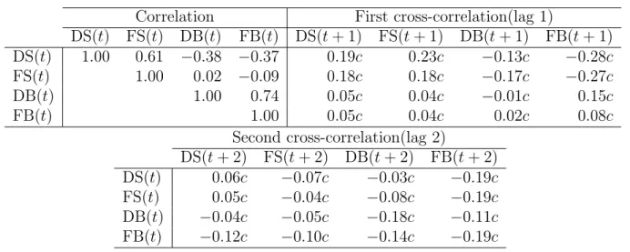
We solve a three-period model for five assets; domestic stock (DS), foreign stock (FS), do-mestic bond (DB), foreign bond (FB) and cash. Foreign currency risk is hedged completely for the foreign assets (FS and FB). Therefore, the rates of return of assets are estimated on a Japanese yen basis. A period is a month. The expected values and standard deviations of rates of asset return and the correlation coefficients among assets are estimated based on the indices from January 2004 to December 2013 as in Tables 3 and 4. The estimated correlation coefficients are the estimates with c = 1 in Table 4. We append the parameter
c because of the sensitivity analysis. We use Nikkei 225 index for the DS, S&P 500 for the
FS, long-term Japanese government bond futures for the DB, and 10-year U.S. Treasury note futures for the FB.
Table 3: Expected values and standard deviations of rates of return
DS FS DB FB
Expected value 0.52% 0.54% 0.04% 0.14%
Standard deviation 5.75% 4.15% 0.84% 2.32%
† Values for foreign assets are on a Japanese yen basis.
16As stated in Hibiki [9], the algorithm used in solving the problem by the hybrid model with the
fixed-proportion strategy also does not guarantee to derive the global optimal solutions because of the similar difficulties.
17Empirically, the objective function value almost converges after two iterations in Step 2 and five iterations
in Step 5 in the numerical analysis after Section 4.2. Therefore we conduct the analysis fixing the number of iterations instead of the convergence condition in Steps 3 and 6. The objective function value in Hibiki [9] converges after two iterations.
18The optimal solutions of the hybrid N4 model can be derived from Steps 1 to 3, and the following Step 4’
instead of the Steps 4 and 5 for the PwL model.
Step 4’ : Set k← k + 1. Wt(k(i)∗−1) is calculated as the amount of wealth of path i at time t of the (k− 1)th iteration. We sort the amount of wealth Wt(k(i)∗−1) at each time and divide m nodes to solve the hybrid Nm model. We solve the problem using the following investment unit function,
h(i)(zsjt) = W (i)∗ t(k−1) ρ(i)jt zs jt.
We calculate the objective function value Objk using the optimal solutions.
The objective function value almost converges after three iterations in Step 4’. Strictly, the degree of freedom of the PwL model is lower than that of the hybrid N4 model because of Equation (3.3). However, we do not discuss the degree of freedom of the models hereafter.
Table 4: Correlation matrices
Correlation First cross-correlation(lag 1)
DS(t) FS(t) DB(t) FB(t) DS(t + 1) FS(t + 1) DB(t + 1) FB(t + 1) DS(t) 1.00 0.61 −0.38 −0.37 0.19c 0.23c −0.13c −0.28c FS(t) 1.00 0.02 −0.09 0.18c 0.18c −0.17c −0.27c DB(t) 1.00 0.74 0.05c 0.04c −0.01c 0.15c FB(t) 1.00 0.05c 0.04c 0.02c 0.08c Second cross-correlation(lag 2) DS(t + 2) FS(t + 2) DB(t + 2) FB(t + 2) DS(t) 0.06c −0.07c −0.03c −0.19c FS(t) 0.05c −0.04c −0.08c −0.19c DB(t) −0.04c −0.05c −0.18c −0.11c FB(t) −0.12c −0.10c −0.14c −0.19c
The interest rates are 0.0214% in the first period, 0.0269% in the second period, and 0.0317% in the third period. These rates are estimated, based on the 1,2,3 month Japanese yen LIBOR interest rates in ten years. Initial amount of wealth is a hundred million yen, and the number of sample paths is 10,000. We calculate CVaR at a 80% confidence level. No short sales are allowed for risky assets, and the upper limit for cash is 10% of total assets. We generate sample paths of asset returns which are assumed to be normally distributed, using the parameters of Tables 3 and 4, and calculate asset prices.19
All of the problems are solved using NUOPT (Ver. 13.1) – mathematical programming software package developed by NTT DATA Mathematical System, Inc. – on Windows 7 personal computer which has Core i5-2540M 2.6 GHz CPU and 8 GB memory.
4.2. Base case
We solve the problems with 0.6 risk aversion (γ = 0.6) and estimated autocorrelation (c = 1) using the PwL model and the hybrid N1, N2 and N4 models, and compare these results. It is expected that the objective function value of the hybrid Nm model is large as m is large because the number of decision variables is almost proportion to the number of decision nodes. As mentioned before, we can compare the PwL model with the hybrid N4 model under the same condition. The objective function values of both models may be similar to each other. The average values derived using the different ten random seeds are shown.
4.2.1. Objective function values and CVaR ratios
We show the optimal objective values derived by four models in the left-hand side of Figure 7. The optimal objective value of the hybrid N4 model is the largest among three hybrid models because we can control risk and return as the number of decision variables increases. The optimal objective value of the PwL model is a little bit larger than that of the hybrid N4 model under the condition of the same number of decision variables. However, we need to pay attention to the fact that the differences are slight among these optimal objective values. It is expected to control risk and return appropriately by employing the PwL investment unit function in terms of wealth as well as the step function in the hybrid N4 model.
In addition, we compare the models using the CVaR ratio in Equation (4.1) expressed
19The interest rates are path-dependent in the formulation. Nevertheless, we assume the interest rates are
by both risk and return measures to evaluate the efficiency of risk-return trade-off. CVaR ratio = E[WT]− W0
CVaR (4.1)
The CVaR ratio measures the excess terminal wealth per unit of CVaR. The higher the investment efficiency is, the larger the ratio is. We show the CVaR ratios in the right-hand side of Figure 7. It is possible to invest in assets efficiently by using the PwL model as well as the hybrid N4 model.
-0.6 -0.5 -0.4 -0.3 -0.2 -0.1
0.0 Hybrid N1 Hybrid N2 Hybrid N4 PwL
ob je ct iv e fu nc ti on v al ue 0.0 0.1 0.2 0.3 0.4 0.5 0.6
Hybrid N1 Hybrid N2 Hybrid N4 PwL
C V aR r at io
Figure 7: Objective function value and CVaR ratio
4.2.2. Asset allocation
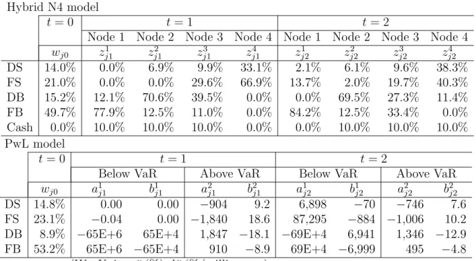
The optimal solutions of the hybrid N4 model are investment weights for each node, while these of the PwL model are the intercept and slope parameters of the PwL function. We show them in Table 5. The cash ratio in the PwL model is derived as one minus the sum of the risky asset ratios.
Table 5: Optimal Solutions Hybrid N4 model
t = 0 t = 1 t = 2
Node 1 Node 2 Node 3 Node 4 Node 1 Node 2 Node 3 Node 4
wj0 zj11 zj12 zj13 zj14 zj21 zj22 zj23 zj24 DS 14.0% 0.0% 6.9% 9.9% 33.1% 2.1% 6.1% 9.6% 38.3% FS 21.0% 0.0% 0.0% 29.6% 66.9% 13.7% 2.0% 19.7% 40.3% DB 15.2% 12.1% 70.6% 39.5% 0.0% 0.0% 69.5% 27.3% 11.4% FB 49.7% 77.9% 12.5% 11.0% 0.0% 84.2% 12.5% 33.4% 0.0% Cash 0.0% 10.0% 10.0% 10.0% 0.0% 0.0% 10.0% 10.0% 10.0% PwL model t = 0 t = 1 t = 2
Below VaR Above VaR Below VaR Above VaR
wj0 a1j1 b1j1 a2j1 bj12 a1j2 b1j2 a2j2 b2j2
DS 14.8% 0.00 0.00 −904 9.2 6,898 −70 −746 7.6
FS 23.1% −0.04 0.00 −1,840 18.6 87,295 −884 −1,006 10.2
DB 8.9% −65E+6 65E+4 1,847 −18.1 −69E+4 6,941 1,346 −12.9
FB 53.2% 65E+6 −65E+4 910 −8.9 69E+4 −6,999 495 −4.8
We show the relationship between the amounts of wealth and the investment weights for three models in Figure 8. The weights at time 1 and time 2 depend on the amounts of wealth, and they are different from those at time 0 in the three graphs on the top of Figure 8. We discuss the characteristics about the asset weights in what follows.
Figure 8: Asset allocation (bold lines show the VaR point)
(1) Time 0
The DB, which is the lowest risky asset, is more invested than the DS and FS, which are higher risky assets in the hybrid N1 model. This reason is in what follows. The adequate investment decision for all paths on average is made after time 1 because the state-dependent decision in terms of wealth cannot be made in the hybrid N1 model. As a result, the most conservative investment strategy is implemented at time 0. This is different from other models. On the other hand, the asset mix of the PwL model is similar to that of the hybrid N4 model. Less investment in the DB and more investments in the DS, FS and FB in the both models are made than the investment in the hybrid N1 model. The reason is that the state-dependent decisions can be made after time 1 for the both models even though their investment unit functions are different each other. If investors have the larger amount of wealth, they adopt the strategy of taking risk to gain higher return at time 1. If they have the smaller amount of wealth at time 1, they adopt the strategy of reducing risk and aiming for the recovery of wealth little by little. Consequently, the riskier asset mix policy is implemented than that of the hybrid N1 model.
(2) Time 1
In the hybrid N1 model, the most conservative investment strategy is implemented as well as time 0. The DB is mainly invested and the weights of stocks (DS and FS) are about 10%. The asset mix at time 1 is almost the same as time 0.
We have the similar asset mixes for both the hybrid N4 model and the PwL model. As the amount of wealth becomes large, the weights of stocks increase and the weights of bonds (DB and FB) decrease. We can afford to invest in stocks because we have much wealth, and attempt to aim the high return.
When the amount of wealth is smaller than the VaR, the optimal weights of DB and FB jump like step functions at the VaR point. The slope parameter of DB (b131 = 65× 104) is positively huge, that of FB (b1
41 =−65 × 104) is negatively huge. We need to constrain the
slope parameters to prevent the optimal weights from jumping at the VaR point.
(3) Time 2
The asset allocations at time 2 are similar to time 1 for all of the models, but the amount of wealth affects the more allocation change at time 2 than time 1. Compared with the results at time 1, stocks are more invested below the VaR point, while bonds are more invested above the VaR point. The asset mix is determined so that the amount of wealth can attempt to exceed the VaR point when it is smaller than the VaR point and it can keep exceeding the VaR point when it is larger than the VaR point.
4.3. Sensitivity analysis
The optimal objective value and the CVaR ratio of the PwL model are a little bit better than the hybrid N4 model in the base case. We conduct the sensitivity analysis for two kinds of parameters; risk averse coefficient (γ) and autocorrelation (c), as follows.
γ : three kinds of risk averse coefficients (γ = 0.6, 0.8,∞) 20
c : five kinds of autocorrelations (c = 0, 0.25, 0.5, 0.75, 1)
4.3.1. Objective function
The objective function values of 15 combinations of γ and c are shown in Figure 9. The objective function is CVaR for risk minimization problem (γ → ∞), and the smaller value is better. ç= 0:6 ç= 0:8 ç! 1㸦risk minimization㸧 -70 -60 -50 -40 -30 -20 -10 0 c=0 c=0.25 c=0.5 c=0.75 c=1 O bj ec ti ve fu nc ti on v al ue Hybrid N1 Hybrid N2 Hybrid N4 Pw Linear -100 -90 -80 -70 -60 -50 -40 c=0 c=0.25 c=0.5 c=0.75 c=1 O bj ec ti ve fu nc ti on v al ue Hybrid N1 Hybrid N2 Hybrid N4 Pw Linear 125 130 135 140 145 c=0 c=0.25 c=0.5 c=0.75 c=1 O bj ec ti ve fu nc ti on v al ue (C V aR ) Hybrid N1 Hybrid N2 Hybrid N4 Pw Linear
Figure 9: Objective function value
We obtain the similar results to the base case. As the autocorrelation parameter (c) becomes large, the objective function value becomes better. This result shows that we can
20The risk averse coefficients (γ) are non-negative. The expected terminal wealth is maximized for γ = 0,
and the CVaR is minimized for γ → ∞. As the risk-averse coefficient becomes large, the risk-averse and conservative strategy is adopted.
take an appropriate investment strategy for asset mix to control the risk-return trade-off according to the existence of autocorrelation.
As the risk-averse coefficient (γ) becomes large, the differences among the models become small. In the risk minimization problem, the CVaR of the PwL model is the smallest, and the CVaR of the hybrid model decreases inversely with the number of decision nodes regardless of the autocorrelation. The reason is that the conservative strategy tends to be adopted as the coefficient γ becomes large. As the results, there are little differences among the models.
4.3.2. Asset allocation
We examine the investment proportion at each time for three kinds of the autocorrelations, and describe the relationship between those and the amount of wealth with γ = 0.6.
(1) Asset allocation at time 0
We show the asset allocation at time 0 in Figure 10.
c=0 c=0.5 c=1 0000000000000000000000000000000 00000000000000000000000000000000000000000000000000000000000000 00000000000000000000000000000000000000000000000000000000000000 000000000000000000000000000000000000000000000000000000000000 0000000000000000000000000000000 0000000000000000000000000000000 0000000000000000000000000000000 0000000000000000000000000000000 0000000000000000000000000000000 0000000000000000000000000000000 0000000000000000000000000000000 0000000000000000000000000000000 0000000000000000000000000000000 0000000000000000000000000000000 0000000000000000000000000000000 0000000000000000000000000000000 0000000000000000000000000000000 0000000000000000000000000000000 0000000000000000000000000000000 0000000000000000000000000000000 0000000000000000000000000000000 0000000000000000000000000000000 0000000000000000000000000000000 0000000000000000000000000000000 0000000000000000000000000000000 0000000000000000000000000000000 0000000000000000000000000000000 0000000000000000000000000000000 0000000000000000000000000000000 0000000000000000000000000000000 0000000000000000000000000000000 0000000000000000000000000000000 0000000000000000000000000000000 0000000000000000000000000000000 0000000000000000000000000000000 0000000000000000000000000000000 0000000000000000000000000000000 0000000000000000000000000000000 0000000000000000000000000000000 0000000000000000000000000000000 0000000000000000000000000000000 0000000000000000000000000000000 0000000000000000000000000000000 0000000000000000000000000000000 0000000000000000000000000000000 0000000000000000000000000000000 0000000000000000000000000000000 0000000000000000000000000000000 0000000000000000000000000000000 0000000000000000000000000000000 0000000000000000000000000000000 0000000000000000000000000000000 0000000000000000000000000000000 0000000000000000000000000000000 0000000000000000000000000000000 0000000000000000000000000000000 0000000000000000000000000000000 0000000000000000000000000000000 0000000000000000000000000000000 0000000000000000000000000000000 0000000000000000000000000000000 0000000000000000000000000000000 0000000000000000000000000000000 0000000000000000000000000000000 0000000000000000000000000000000 000000000000000000000000000000 000000000000000000000000000000 000000000000000000000000000000 000000000000000000000000000000 000000000000000000000000000000 000000000000000000000000000000 000000000000000000000000000000 000000000000000000000000000000 000000000000000000000000000000 000000000000000000000000000000 000000000000000000000000000000 000000000000000000000000000000 000000000000000000000000000000 000000000000000000000000000000 000000000000000000000000000000 000000000000000000000000000000 000000000000000000000000000000 000000000000000000000000000000 000000000000000000000000000000 000000000000000000000000000000 0% 10% 20% 30% 40% 50% 60% 70% 80% 90% 100% W ei gh ts 000000000000000 000000000000000FB 0.00% 0.00% 0.00% 0.00% 000000000000000 000000000000000DB 89.27% 88.91% 88.48% 88.37% 000000000000000 FS 1.98% 2.16% 2.59% 2.76% DS 8.75% 8.92% 8.94% 8.87% Cash 0.00% 0.00% 0.00% 0.00% Hybrid N1 Hybrid N2 Hybrid N4 Pw Linear
0000000000000000000000000000000 0000000000000000000000000000000 00000000000000000000000000000000000000000000000000000000000000 00000000000000000000000000000000000000000000000000000000000000 0000000000000000000000000000000 0000000000000000000000000000000 0000000000000000000000000000000 0000000000000000000000000000000 0000000000000000000000000000000 0000000000000000000000000000000 0000000000000000000000000000000 0000000000000000000000000000000 0000000000000000000000000000000 0000000000000000000000000000000 0000000000000000000000000000000 0000000000000000000000000000000 0000000000000000000000000000000 0000000000000000000000000000000 0000000000000000000000000000000 0000000000000000000000000000000 0000000000000000000000000000000 0000000000000000000000000000000 0000000000000000000000000000000 0000000000000000000000000000000 0000000000000000000000000000000 0000000000000000000000000000000 0000000000000000000000000000000 0000000000000000000000000000000 0000000000000000000000000000000 0000000000000000000000000000000 0000000000000000000000000000000 0000000000000000000000000000000 0000000000000000000000000000000 0000000000000000000000000000000 0000000000000000000000000000000 0000000000000000000000000000000 0000000000000000000000000000000 0000000000000000000000000000000 0000000000000000000000000000000 0000000000000000000000000000000 0000000000000000000000000000000 0000000000000000000000000000000 0000000000000000000000000000000 0000000000000000000000000000000 0000000000000000000000000000000 0000000000000000000000000000000 0000000000000000000000000000000 0000000000000000000000000000000 0000000000000000000000000000000 0000000000000000000000000000000 0000000000000000000000000000000 0000000000000000000000000000000 0000000000000000000000000000000 0000000000000000000000000000000 0000000000000000000000000000000 0000000000000000000000000000000 0000000000000000000000000000000 0000000000000000000000000000000 0000000000000000000000000000000 0000000000000000000000000000000 0000000000000000000000000000000 0000000000000000000000000000000 0000000000000000000000000000000 0000000000000000000000000000000 0000000000000000000000000000000 0000000000000000000000000000000 0000000000000000000000000000000 0000000000000000000000000000000 0000000000000000000000000000000 0000000000000000000000000000000 0000000000000000000000000000000 0000000000000000000000000000000 0000000000000000000000000000000 0000000000000000000000000000000 0000000000000000000000000000000 0000000000000000000000000000000 0000000000000000000000000000000 0000000000000000000000000000000 0000000000000000000000000000000 0000000000000000000000000000000 0000000000000000000000000000000 0000000000000000000000000000000 0000000000000000000000000000000 0000000000000000000000000000000 0000000000000000000000000000000 0000000000000000000000000000000 0000000000000000000000000000000 00000000000000000000000000000000000000000000000000000000000000 0000000000000000000000000000000 0% 10% 20% 30% 40% 50% 60% 70% 80% 90% 100% W ei gh ts 00000000000000 00000000000000FB 0.00% 1.82% 6.56% 7.45% 00000000000000 00000000000000DB 88.57% 85.15% 78.19% 76.88% 00000000000000 FS 4.69% 6.22% 9.09% 9.26% DS 6.74% 6.81% 6.16% 6.42% Cash 0.00% 0.00% 0.00% 0.00% Hybrid N1 Hybrid N2 Hybrid N4 Pw Linear
0000000000000000000000000000000 0000000000000000000000000000000 0000000000000000000000000000000 0000000000000000000000000000000 0000000000000000000000000000000 0000000000000000000000000000000 0000000000000000000000000000000 0000000000000000000000000000000 0000000000000000000000000000000 0000000000000000000000000000000 0000000000000000000000000000000 00000000000000000000000000000000 00000000000000000000000000000000 00000000000000000000000000000000 00000000000000000000000000000000 00000000000000000000000000000000 00000000000000000000000000000000 0000000000000000000000000000000 0000000000000000000000000000000 0000000000000000000000000000000 0000000000000000000000000000000 0000000000000000000000000000000 0000000000000000000000000000000 0000000000000000000000000000000 0000000000000000000000000000000 0000000000000000000000000000000 0000000000000000000000000000000 0000000000000000000000000000000 0000000000000000000000000000000 0000000000000000000000000000000 0000000000000000000000000000000 0000000000000000000000000000000 0000000000000000000000000000000 0000000000000000000000000000000 0000000000000000000000000000000 0000000000000000000000000000000 0000000000000000000000000000000 0000000000000000000000000000000 0000000000000000000000000000000 0000000000000000000000000000000 0000000000000000000000000000000 0000000000000000000000000000000 0000000000000000000000000000000 0000000000000000000000000000000 0000000000000000000000000000000 0000000000000000000000000000000 0000000000000000000000000000000 0000000000000000000000000000000 0000000000000000000000000000000 0000000000000000000000000000000 0000000000000000000000000000000 0000000000000000000000000000000 0000000000000000000000000000000 0000000000000000000000000000000 0000000000000000000000000000000 0000000000000000000000000000000 0000000000000000000000000000000 00000000000000000000000000000000 00000000000000000000000000000000 00000000000000000000000000000000 0000000000000000000000000000000 0000000000000000000000000000000 0000000000000000000000000000000 0000000000000000000000000000000 0000000000000000000000000000000 0000000000000000000000000000000 0000000000000000000000000000000 0000000000000000000000000000000 0000000000000000000000000000000 0000000000000000000000000000000 0000000000000000000000000000000 0000000000000000000000000000000 0000000000000000000000000000000 0000000000000000000000000000000 0000000000000000000000000000000 0000000000000000000000000000000 0000000000000000000000000000000 00000000000000000000000000000000 00000000000000000000000000000000 00000000000000000000000000000000 00000000000000000000000000000000 00000000000000000000000000000000 00000000000000000000000000000000 00000000000000000000000000000000 00000000000000000000000000000000 00000000000000000000000000000000 00000000000000000000000000000000 00000000000000000000000000000000 00000000000000000000000000000000 00000000000000000000000000000000 0% 10% 20% 30% 40% 50% 60% 70% 80% 90% 100% W ei gh ts 000000000000000 000000000000000FB 0.36% 15.93% 49.73% 53.22% 000000000000000 000000000000000DB 87.84% 66.08% 15.20% 8.91% 000000000000000 FS 3.96% 7.56% 21.04% 23.06% DS 7.83% 10.43% 14.03% 14.81% Cash 0.00% 0.00% 0.00% 0.00% Hybrid N1 Hybrid N2 Hybrid N4 Pw Linear
Figure 10: Asset allocation at time 0
In the case of c = 0, there are little different among four models. But as the autocorre-lation parameter (c) becomes large, the weights of stocks (DS and FS) become large and we can find the explicit difference among these models. As stated above, the autocorrelation parameters affect the asset mix so that the objective function value can be improved.
(2) Asset allocation at time 1 and time 2
We show the asset mixes at time 1 in Figure 11 and time 2 in Figure 12 for the hybrid N4 model and the PwL model. They vary with the different autocorrelations.
When the amount of wealth is larger than the VaR point, the weights of the PwL model are also similar to the weights of the hybrid N4 model as well as the results of the base case. The weights of stocks become large, and the weights of bonds become small as the parameter c is large. We take risk by employing autocorrelations among assets. In addition, the weights of stocks at time 2 are smaller than those at time 1. We do not need to take risk at time 2 when the amount of wealth is larger than the VaR point.
When the amount of wealth is smaller than the VaR point, the optimal weights of DB are more than 80% at time 1 and 70% at time 2 in the hybrid N4 model. The decisions are conservative because four nodes are divided at 25%, 50%, 75% points, and the simulated paths below the 80% VaR point belong to the same node. On the other hand, the optimal weights of FB, DS, and FS in the PwL model become larger than those in the hybrid N4 model. We can control investment decisions in the PwL model.
Figure 11: Asset allocation at time 1
5. Concluding remarks
In this paper, we propose the PwL model for state-dependent asset allocation with CVaR to solve the multi-period portfolio optimization problem in the simulated path approach. We can provide investment strategies with the PwL function, rather than the step function of the asset weights in terms of wealth. It is very useful for investors who manage their multiple assets dynamically. We conduct the sensitivity analysis for the several risk averse coefficients and autocorrelations, and we examine the usefulness of the model through detailed analyses.
In the future research, we need to study the following problems.
(1) The PwL function proposed in this paper is kinked only at the VaR point. We may need to increase the number of kinked points to express the state-dependent function precisely.
(2) The PwL function is dependent on only the amount of wealth. We may need to introduce the other state variables to express the state-dependent function.
(3) We need to evaluate the performance by using practical or out-of-sample data.
(4) We attempt to examine the results in the various cases of the complicated stochastic process, and so on.
(5) We need to clarify the forms of the state-dependent functions for other risk measures by using the hybrid model with a lot of decision nodes.
References
[1] E. Bogentoft, H. Romeijn, and S. Uryasev: Asset/Liability Management for Pension Funds Using CVaR Constraints. The Journal of Risk Finance, 3-1 (2001), 57–71. [2] G. Calafiore: Multi-period Portfolio Optimization with Linear Control Policies.
Auto-matica, 44 (2008), 2463–2473.
[3] J. Cvitani´c and I. Karatzas: On Dynamic Measures of Risk. Finance and Stochastics.
3-4 (1999), 451–482.
[4] J. Detemple, R. Garcia, and M. Rindisbacher: Simulation Methods for Optimal Port-folios. In Birge, J. R. and V. Linetsky (eds.): Handbooks in Operations Research and
Management Science: Financial Engineering Volume 15 (Elsevier, 2007), 867–924.
[5] N. Hibiki: Multi-period Stochastic Programming Models Using Simulated Paths for Strategic Asset Allocation. Journal of Operations Research Society of Japan, 44 (2001), 169–193 (in Japanese).
[6] N. Hibiki: A Hybrid Simulation/Tree Multi-period Stochastic Programming Model for Optimal Asset Allocation. In H. Takahashi (eds.), The Japanese Association of
Financial Econometrics and Engineering, JAFEE Journal [2001], 89–119 (in Japanese).
[7] N. Hibiki: Numerical Analysis for Multi-period Stochastic Programming Models Using Simulated Paths. The Proceedings of the 18th Conference on the Japanese
Associa-tion of Financial Econometrics and Engineering (JAFEE, Tokyo, 2002), 203–214 (in
Japanese).
[8] N. Hibiki: Hybrid Simulation/Tree Stochastic Optimization Model for Dynamic Asset Allocation. In B. Scherer (eds.), Asset and Liability Management Tools: A Handbook
for Best Practice (Risk Books, 2003), 269–294.
[9] N. Hibiki: Multi-period Stochastic Optimization Models for Dynamic Asset Allocation.