Research in Semi-Markovian Decision Structures

(1)

Journal of the

Operations Research

Society of Japan

VOLUME 6 Augut 1964 NUMBER 4

---Introduction

RESEARCH IN SEMI-MARKOVIAN

DECISION STRUCTURES

RONALD A. HOWARD

Operations Research Genter Massachusetts Institute of Technology

The complexity of modern management problems requires correspondingly sophisticated models for management systems. We shall here discuss a statistical model useful in analyzing a wide variety of common problems, problems in the areas of maintenance, replacement, marketing, finance, and inventory control, for example. This model has been under continuing development at M. I. T. for some years. Its present form is the result of encountering practical situations that required successive generalizations of the model.

The basis for the present model is a decision model developed for strictly Markov processes1--processes that satisfy the Chapman-Kolmogorov equations. These processes can be characterized as processes in which the main interest is on state transitions rather than on the time required for a transition. The time between transitions can be considered very easily if transitions occur at regularly spaced points of time or if the times of transition are exponentially distributed. The case of regularly spaced transitions occurs frequently in practice because many decisions are made on a weekly, monthly, or annual basis. The case of exponential transition times, how-ever, does not seem to arise very often.

(2)

164 Ronald A. Howard

The desire to allow other types of transition behavior was encouraged by the development of the semi-Markov process2_,S,4._{This process allowed the time between}

transitions to be a random variable conditional on the transition made. The decision model for the strictly Markov process had interesting properties primarily because its structure involved only the limiting state probabilities of the Markov process. When it was noted that a semi-Markov process had the same limiting state proba-bilities as an exponential Markov process with the same mean times for transitions, it was natural to expect that the decision model could be extended to the semi-Markov process. In this paper we shall point out some of the results of this development and show how this increase in generality does not exact a computational penalty.

*

Setni-Markov Processes

Let us begin by defining those parts of semi-Markov process theory that we shall need. Consider a process with N states. Let

Pi}

be the conditional probability that the next transition is to state} given that the last transition was to state i. We shall call these probabilities the transition probabilities; they must satisfy the condi-tions N

L:

Pij=

1 j=l

P020

i=I,2, ... ,N lsi, }-sN (1) (2)

Whenever a process enters a state, we imagine that it selects from these probabilities to determine the next state to which it will move. However, before making this transition, it "holds" for a time T if in state i where i is the index of the present state and} that of the state selected as its next state. The quantities T if are random variables governed by a corresponding set of density functions, hi} (.), l-si,j-sN. These density functions are called the "holding time" density functions. In general we must specify N2 of them to determine a semi-Markov process. After holding in state i for the time T if the process makes the transition to} and then repeates the whole procedure.

We see that, if we ignore the random nature of transition times and focus on

*

Some of the results in this paper were also discovered independently by]. de Cani

(University of Pennsylvania), W. S.]ewell (University of California, Berkeley) and P. Schweitzer (Massachusetts Institute of Technology).

(3)

Research in Semi-Markovian Decision Structures 165 the transition instants, the process is an ordinary Markov process. However, when the hold behavior is included the process will not satisfy the Chapman-Kolmogorov equations unless the holding times are all exponentially distributed. Therefore the process is Markovian only at the transition instants; hence the name "semi-Markov" process.

We shall find it useful to develop additional notation for the holding time behavior. We shall use chu(.) for the cumulative probability distribution of 1'ij'

(3)

and cChij(.) for the complementary cumulative probability distribution of 1'ij, (4)

We shall assume that the means f i j of all the holding time distribution are finite and that all the holding time density functions have no impulse component at the origin. Suppose now that the process enters state i and chooses its successors state j, but that we as observers do not know the successor chosen. The density function that we would assign to its holding time in i, r i> would then be wJ.), where

(5)

We shall call this function the unconditional waiting time density function for state i. The mean unconditional wait in state i, ;f i' is related to the means of the holding times for state i by

(6)

The cumulative and complementary cumulative probability distributions for the unconditional wait are given by

(7)

(4)

When modeling real systems with semi-Markov processes we must decide whether we want to call a movement from a state to itself a transition of the process. We find it convenient to make the decision different ways in different circumstances. To distinguish we shall say that the system makes a "real" transition only when its state number actually changes, but that it makes a "virtual" transition when it re-enters the same state. Some models require that only real transitions be allowed, in others the virtual transitions are the most important. For example, if we are studying a machine maintenance problem in which the state of the system is the number of machines working, then only real transitions need be considered because a virtual transition would require a simultaneous breakdown and repair. On the other hand in a marketing problem the state variable might be the last brand purchased by the customer. In this case virtual transitions would correspond to repeat purchases of the same brand, a very important phenomenon. In our development we shall allow the possibility of virtual transitions; the diagonal transition probabilities Pii mayor may

not be zero.

Now let us proceed to the question of state probabilities for a semi-Markov process. Let ifJij Ct) be the probability that the system is in statej at time t given that

it entered state i at time zero. We shall call these probabilities the interval transition probabilities of the process. We can write a recursion equation for ifJij Ct) as follows.

A system starting in state i can be in statej at time t either because i = j and it never left i during that interval or because it left i at least once and finally managed to reachj by time t. The probabilities of these two mutually exclusive possibilities are added in this equation,

i=j i~j

l:::;:i, j:::;:N; t~O (9)

The quantity

0iJ

assures that the term in which it appears occurs only when i = j. The complementary cumulative probability cc_Wi Ct) is the probability that the system will not leave its starting state i until after time t. The second term in the equation represents the probability of the sequence of events where the system

(5)

Research in Semi-Markovian Decision Structures 167

makes a transition from i to some state k (maybe itself) at time r and then proceeds to state j from k in the remaining time t - 7:. This probability is summed over all states k to which the initial transition could have been made and integrated over all times of transition r between 0 and t.

Solving this recurrence equation in its present form is not particularly easy. However, exponential transformation simplifies it considerably. Let

(10)

be the exponential transform of the function f(t). Then we find the exponential transform of Equation 9 to be

l~i, j~N. Cll)

Since from Equation 8,

(12)

the exponential transform of the complementary cumulative waiting time distribu-tion in state i is

(13)

Equation 11 now relates the transform of the interval transition probabilities to the basic process quantities.

A matrix formulation of Equation 11 will prove worthwhile. We shall define matrix of any double-indexed quantity to be the corresponding upper case letter. Thus 0(t) = {s6il(t)}, P={Pu}' etc. We shall also define diagonal matrices W(t) = {OilWi(t)}, CW(t) = {OijcWi(t)}, and cCW(t) = {o;/CWi(t)}. The special form of the summation in Equation 11 makes it worthwhile to define a special kind of matrix multiplication designated by

D .

If A, B, and Care N by N square matrices, then C = A DB implies cij = 02iJbij, l~ i, j ~N. In other words the "box" operation is an element by element multiplication.

(6)

168 Ronald A. HOlDard

Now we can write Equation 11 in the form

(14)

The transform of the interval transition probability matrix (/J T(S) is thus

(15)

The inverse matrix will always exist for the type of process we are considering. We see that the interval transition probabilities depend only on the products of

Pu

and hij(t), not on the individual quantities.

Equation 15 provides the means for relating the interval transition probabili-ties of a semi-Markov process to the process parameters. However, for the purposes of this paper we shall not need to explore the transient behavior of interval transition probabilities, but only their limiting form. Let us define a limiting interval transition probability matrix for the process by

(/J=lim(/J(t). (16)

t+~

By the final value theorem of exponential transforms (/J is also given by

(/J=lim s (/JT(S). (17)

HO

We use Equation 15 to write this limit in the form

(/J=lims (/JT(s)=lims [I-PDHT(s)]-llimCCWT(s). (I 8)

'+0 '+0 '+0

We now consider each of the limits on the right of Equation 18 individually. First, by Equation 13,

(19)

where I is the identity matrix. However, because WT(O) = I, the limit is indetermi-nate and we must resort to L'Hospital's rule. We find

limcCWT(s)=-+WT(S)i = f''''t W(t)dt=M.

'+0 s 8=0 0

(20)

The matrix M is therefore a diagonal matrix of the mean unconditional waiting times in each of the states of the process.

(7)

Research in Semi-Markovian Decision Structures 169 Now we find the other limit in Equation 18,

lim s [I -P

0

HT(s)]-l=lim T(s). (21) 8-+0 8-+0

where we have written T(s) for s times the inverse matrix. Then T(s) =s [I -1'

0

HT(s)l-1

or

T(s) - T(s) P [] HT(S) = sI. (22)

If we take the limit of Equation 22 as s approaches zero and note that HT(O) is a matrix with all elements equal to one, we obtain

T(O) = T(O)P. (23)

We shall now show that the rows of the T(O) matrix must be proportional to the limiting state probabilities of the imbeddecl Markov process that describes the transi-tions of the process without respect to their duration. Let us suppose in the remainder of this paper that this imbedded Markov process has only one recurrent chain and therefore a unique set of limiting state probabilities independent of the starting state. What we shall say about this case can be extended fairly easily to the multiple chain problem. Let 11:i be the limiting probability of state i for the imbedded process. Then

these probabilities must satisfy the equation,

N 11:j =

1:

11:iPij, i=l N

1:

11: i

=1.

(24) i=I

Since the solution is unique for a single chain process, the rows of the T(O) matrix must each be proportional to the row vector IT with elements 11:j •

We have now reduced Equation 1B to the form

f/>= T(O) M. (25)

The elements of f/> must therefore satisfy

(26)

where ki is an undetermined constant of proportionality between the ith row of T(O)

(8)

170 _{Ronald A. Howard}

use the condition that the limiting interval transition probabilities

rpo

must sum to one over all the states of the process. Thus

(27)

and therefore

(28)

The constant of proportionality is then the same for all states and we can write from Equation 26 and 28,

(29)

As we would expect, the limiting interval transition probabilities

rpo

do not depend on the starting state i. We shall, therefore use only the second subscript to indicate these quantities. Furthermore, these probabilities are equal to the limiting state pro-babilities of the imbedded Markov process weighted by the mean unconditional waiting times in each state. This result is intuitive and important: the only statistic of each holding time distribution that affects the limiting behavior of the process is its mean.

A Reward Structure

We shall now superimpose on the semi-Markov process a system of rewards. The system will earn both by making transitions and by staying in a state. Let TU be the transition reward for a transition from state i to statej. It is a lump sum quantity paid when the transition occurs. Let Yi be the yield rate for state i, the amount the system will earn per unit time for all the time it stays in state i. A large class of physical processes can be modeled by this type of reward structure or by simple variations of it. For example, a machine maintenance system whose state was the number of machines in operation might earn profit at a rate corresponding to the number of operation and incur a fixed charge whenever a breakdown occurs.

(9)

Research in Semi-Markovian Decision Structures 171 we expect the system to earn in a time t if it enters some state, say state i, at time zero; let this quantity be represented by vi(t). The system will either stay in i throughout the time t or else make a transition out of state i (but possibly to enter state i again ill a virtual transition). If the system stays in state

i

for the entire interval, then it will earn the yield rate Yi multiplied by the time t. It will also earn whatever terminal reward may be associated with being in state i at the end of the time t, a quantity we shall denote by Vi(O). Such a terminal reward may be extremely important in certain systems where scrap value or another such terminal cost must be included in the for-mulation. The probability that the system will not leave state i during the interval is just CCWi(t). Therefore the contribution to the expected total reward vi(t) due to

the possibility of the system's not leaving state i is cCWi(t )[vi(O)

+

Yit).

,. The system may leave state i for some state'; at some time 7: between zero and t. If it does so it will earn transition reward rij, and the yield rate Yi for a time 7:.

However, it will also be in a position to earn whatever expected reward is associated with entering statej when a time t-7: remains in the process, Vj(t-7:). The sum of these quantities must be multiplied by the probability that the system will make its necessary transition to statej,

Aj,

and by the probability density function of the hold time for this transition evaluated at the point 7:, h;j(7:). The result must then be summed over all states j in the system and integrated over all values of 7: between 0 and t. When these operations have been performed we obtain as the final expression for the expected total reward,

Vi(t) =ccWi(t{Vi(O)

+

Yi t ]

+

t/iJ

f>7:h

u

(7:) [ru

+

Yt7:+Vj(t -7:)

J.

i=I,2, ... ,N; t20. (30)

Equation 30 provides a method for calculating total expected rewards for any starting state and any time period. However, the calculation is involved for all but the simplest cases. The numerical analysis required to solve the equation essentially reduces the problem to that of the fixed transition time Markov process because of the necessity of considering discrete time increments. Consequently, we shall focus our interest here on the behavior of this equation in the situation where t is very large; that is, where the process is going to be allowed to run for a relatively long

(10)

time. Fortunately, the behavior we shall study is of practical importance in most processes after only a few transitions are made.

When t is very large CCWi(t) approaches zero because we are concerned only with systems having finite mean holding times. Furthermore, it is easy to show that t CCWi(t ) approaches zero as well. Therefore when t is very large in Equation 30

i = 1,2, ... , N; for t large (3 I)

or

i = 1,2, ... , N; for t large (32) Let us use a quantity qi defined by

i=I,2, ... ,N (33)

and call it "earning" rate in state i to simplify Equation 32. We can then write vJt) =q/fi

+~/ijf:

drhij(Th (t -T)

i=I,2, ... ,N;fortlarge (34)

By the basic Equation 30 it is possible to show that when t is large Vi(t) has the form

i=I,2, ... ,N; fortlarge. (35) Indeed, all of our present results can be obtained rigorously, if somewhat laboriously, by transform methods. However, the present development will illustrate the properties we need. Equation 35 says that the expected reward will grow linearly with t when t is large. The growth rate is g, a quantity that we call the gain of the process. The gain is thus the average reward per unit time that the system will earn in the steady state. As we would expect it is independent of the state in which the system is started.

(11)

Research in Semi-Markovian Decision Structure:

vi+gt=q/r i +

f

Pilf'" dThij('r) [Vj+ (t-T)g]

)=1 0 N =q;'fi

+

L.PUVj+gt-gri. j=1 173 (36)

The quantity gt appears on both sides of this equation and therefore vanishes. We have thus found that for large t,

.Y

Vi

+

gfi =qifi

+

L.

PUVj

j=I

i=I,2, .. . ,N (37)

Equation 37 allows us to solve for the gain of the process m terms of the transition probabilities and the mean unconditional waits in each state. The equation is homogeneous in the v/s; we can set one of the quantities Vi arbritrarily. We shall use this freedom to set V N = O. Then for the type of process we are considering, the remaining values will be determined by these equations to within a constant as a direct result of solving the equations implied by expression 37. We can therefore find the gain of the process and also a set of quantities that differ from the quantities Vi by the same constant. We shall find that the solution of these equations plays a central role in the decision structure we shall soon add.

There is another result obtained quite readily from Equation 37. First we multiply this equation by the limiting state probability for state i in the imbedded Markov process and then sum the result for all values of i. The result is

(38)

From Equation 24 we see that the first and last terms of this equation are equal. It reduces to or N N g

L. 7'C

i f i ,=,

L.

7'C_iqif i i=l i=l N

L.

7'C ifi Qi g = -"c::.

=+'1--L.7'C

ifi i "'1 (39) (40)

(12)

174 Ronald A. HOlDard

Now if we apply Equation 29 we can write

(41)

The gain of the process is just the sum of the earning rates for each state weighted by the limiting interval transition probabilities for the process. This result is consistent with our intuition about the process.

The semi-Markov process with a reward structure is an excellent model for several stochastic processes. It offers a method by which general results can often be obtained with little difficulty. For example, consider the problem of establishing the order quantity

0.

for an inventory system with the following characteristics. A single item is subject to random demand with the time between succeeding demands selected independently from the same probability density function; mean time between de-mands is 1/).. No stockouts are permitted, lead time is zero, there is a fixed cost A of placing an order, and a carrying charge of r per unit time to be assessed against each item in inventory. We see that we can model this inventory system as a semi-Markov process whose state index i represents the number of items in inventory at any time. The state index can range from 1 to

0.

,the order quantity. It cannot be zero because when the last item in inventory is sold the amount of stock in inventory jumps instant-aneously to

0..

The transition probability structure is therefore very simple: the imbedded Markov process is periodic with period

0..

The state index falls by one unit with each transition (demand) unless there is only one unit in inventory in which case it become

0..

Therefore the limiting state probability for each state in the imbedded Markov process is just

1/0.,

7ri=

1/0.

i=1,2, ... ,0..

The holding time in every state is the density function of time between demands. The mean holding time in any state is therefore

i=I,2, ... ,0..

Since the expected holding time in all states is the same, we see from Equation 29 that the limiting interval transition probabilities

1>i

will be equal to the limiting

(13)

Research in Semi-Markovian Decision Structures 175 state probabilities ~ i,

i=I,2, ... ,Q.

The reward structure for this example is also simple. Since this system can only lose money we shall deal in costs rather than rewards. There is no transition cost associated with any transition except the transition from state I to state Q. The cost associated with this transition is the ordering cost,

otherwise

The yield rate in any state is the inventory carry charge rate of that state. For state i this will be ir,

Yi=ir i,=1,2, ... ,Q.

We can now calculate the earning rate in each state using Equation 33 and these results. We find

i =1,2, .. .

,Q,

i=2,3, ...

,Q.

Now that we have obtained both the limiting interval transition probabilities and the earning rates for the system we can use Equation 41 to write the gain, which in this case is the average cost per unit time of operating the system in the steady state. We find

=

d.

[AA

+

r

~,

iJ

=

d.

[AA

+

r

Q

(%

+

1)

J

=~+ r(Q+O

(14)

Now all that remains is to find the value of Q that minimizes this average cost rate. If we ignore the discrete nature of Q, differentiate g with respect to Q and set the derivative equal to zero, we find that the minimizing

Q

is given by

which is, of course, the famous Wilson lot-size formula. The best integral value of Q can be found by difference methods if necessary.

Note that the generality of the semi-Markov process has allowed us to establish this result for demand processes that range from Poisson to constant time between purchases. Such modifications as quantity-dependent ordering costs and inter-demand distributions that depend on the inventory level would complicate the model only slightly. Even the problem of multiple-demands occurring at the same time can be treated. The freedom to expand the problem under consideration in several interest-ing ways at small increase in difficulty is a particularly appealinterest-ing feature of st'mi-Markov models.

A Decision Structure

Suppose now that when the system is in state i there are various alternatives for its operation. Associated with the kth alternative in state i are all the process para-meters:

pL,

h}j ( .), .y}, and rfj. They are given a superscript k to indicate this association. Thus if a system enters state i and follows alternative k in that state, the next transition that will be made, the time of that transition, the yield rate for occu-pancy of state i, and the reward for the transition to the next state will all be governed by the alternative. We shall assume that the alternatives available are finite but that they may be different in number from one state to another. The problem we pose is this. Suppose we are free to select one alternative in each state for the operation of the system. We shall call such a selection in anyone state a decision and in all states a policy. The policy once established will be fixed for all time-every time the system enters a state it will follow the alternative dictated by the policy. The problem is now simply stated: Find the policy that maximizes the gain (average reward per unit time in the steady state) for the system.

(15)

Research in Semi-Markooian Decision Structures 177 As in the case of strictly Markovian processes, the solution can be found by an iteration scheme. We shall first establish its plausibility and then prove that it works. If we solve Equation 37 for g, we obtain

i=1,2, .. . ,N. (42)

It seems reasonable that to maximize g we want to make the right hand side of this equation as large as possible. That is exactly what we do in the iteration scheme. We begin with an arbitrary policy for the system and then solve Equation 37 to determine the gain of this policy and the quantities Vi which we shall call the relative values. Then we use these

v;'s

to improve our policy by finding the alternative in each state i that maximizes the test quantity

(43)

We shall not change the old decision unless another alternative has a strictly greater value of the test quantity. When a new decision (possibly the same) has been made in each state, a new policy has been found. Note that the relative nature of the

v;'s

does not affect the policy improvement process because the test quantity, expression

43, is unchanged if any constant is added to all the v/so The test quantity involves the transition probabilities of each alternative, pfj, the mean unconditional holding time in state i under that alternative,

f:'

and the earning rate it prescribes for state i, q}. The earning rate for the alternative is in turn defined by Equation 33 as

i=I,2, .. .. N. (44)

Consequently we see that the holding time density functions enter into the calcula-tions only through their means. We do not find this result surprising because we al-ready know that the limiting interval transition probabilities for the semi-Markov process depend only on the same characteristics of the holding time density functions and because the gain depends only on the earning rates and the limiting interval transition probabilities.

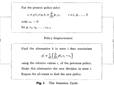
The iteration cycle is shown in Fig. I. We select an arbitrary policy and evalu-ate it in the upper box in the figure. Then we enter the policy improvement box with

(16)

the relative values for this policy and find the alternative in each state that maximizes the test quantity. When we have performed this operation for all states in the system, a new policy has been found. We shall soon show that this policy can only increase in gain as a result of the policy improvement operation. The iteration terminates when the policy on two successive cycles is identical.

Let us illustrate the type of calculation involved with an example. Suppose that a machine facility can be in either of two states. It is in state 1 when the machine is operating and in state 2 when the machine is out of order. When the machine is in state 1 it can be maintained with either normal or expensive maintenance; these two options are the two alternatives in state 1. Under either maintenance policy the machine will sooner or later break down so that

prl

= 0, pf2 = 1 for either alternative. However, the density function of time until the next breakdown will be different in each case. Under alternative 1, normal maintenance, the time to breakdown will have the density function hI2(t) = 5e-5L

• Under alternative 2, expensive maintenance,

it will be h~2(t) = 16te-4t

• The yield rate for normal maintenance will be larger than

1-I ~_I

\

I

I ' Policy Evaluation

---For ~h-e-I~rese~t;o-I-ic-y-SO-I-v-e--- -

----I

N

v,+gf,=q,f,+

2:

PUVj

j=l

i=I,2 •...• N

Policy Improvement

Find the alternative k in state i that maximizes

using the relative values v, of the previous policy. Make this alternative the new decision in state i.

Repeat for all states to find the new policy. Fig. 1 The Iteration Cycle

(17)

under expensive maintenance because of the higher maintenance cost; in fact,yt = 6,

)'~ = 4. There is no transition reward associated with the transition from state 1 to state 2.

When the system is in state 2 and the machine is out of order, there are again two alternatives, inside-plant and outside-plant repair crews. Under either alternative, the machine will sooner or later be fixed: P~l = 1, P~2 = O. The time for the repair, h~l(t) = 64te-8t_; _{for outside repair it is}_Izll(t)₌ _7e-7t_•_{There is a fixed charge of 0.5}

for restarting the machine after either repair, and a charge per unit time of 1 for the inside crew and 1.5 for the outside crew: r~l = r~l = -0.5,.y~ = -l,y~ = -1.5.

The data for the example are summarized in Table I. The mean time to the next transition under each alternative is of particular interest. We see that the effect of the more expensive maintenance is to increase the expected time until the next breakdown, and that the effect of using the outside repair crew is to shorten the expected time for completion of the repair. The earning rates for each state and alter-native calculated using Equation 44 also appear in the table. One way of finding the policy that maximizes the gain of the process would be first to find the limiting interval transition probabilities for each of the 4 possible policies in this problem by

State Alternative k 2 2 I 2 k ro -0.5 -0.5 Transition Probabilities r~2 0 0

Holding Time Densities M.(t) Yield Rates 6 4 - I -1.5

o

Earning Rates 6 4 -3 -5 Table I. A Machine Repair Example

Mean Uncondi-tional Waits liS 1/2 1/4 1/7

(18)

180 Ronald A. Howard

using Equation 29 with 1l"1 =1l"2 = 1/2. Then we could use Equation 41 to find the

gain of each policy and finally choose the one with the maximum gain. This procedure is feasible for this problem, but not for even a slightly larger one because the number of possible policies grows very quickly. The iteration method is valuable because it can treat problems that would be difficult to solve by exhaustion.

We begin the iteration procedure by choosing a policy arbitrarily. A conven-ient first choice is the policy that maximizes the earning rate in each state. In this example it is the policy formed by the first alternative in each state. We shall denote a policy by a column vector rJ. whose ith element is the alternative selected in the ith

state. Therefore the initial policy is described by

1=UJ.

We now write the policy evaluation equations 37 for this policy,

VI

+

1/5g=6/5+v2

v2

+

1/4g= -3/4+v1

(45)

(46)

When we set V 2 = 0, we find immediately, g = 1, VI = 1. The gain of the system under the initial policy is 1 per unit time.

Now we try to improve the policy by maximizing the test quantity 43 in each state using the values VI = I, V 2 = O. The calculations involved appear in Table 11.

State Alternative k 2 2 2 Test Quantity

qH

-h

[£

P~,vJ

- VJ]

't'i }=1 6+5(-1) = 1 4+2(-1) = 2 -3+4(1) = 1 -5+7(1) = 2 Table IT. Policy Improvement for Machine Repair Example

We see that the second alternative in each state now has the higher value of the test quantity. Therefore the policy is changed to

(19)

We now solve the policy evaluation equation for this policy both to assure ourselves that the gain has, in fact, increased and to provide the relative values Vi required

for possible further improvement. The equations are v, +lj2g=,2+v2

v2+1j7g=' -5/7+v, . (48)

With V2 = 0 we obtain the solution g = 2, VI = 1. The gain.has doubled to 2 per

unit time. Ifwe now attempt policy improvement we see that we are going to repeat the calculations in Table II because VI and _V2have the same values as before.

There-fore the policy found by the second alternative in each state has the highest gain of any policy in the system; the iteration has converged.

The management of the machine facility should therefore find it most profit-able in the long run to use expensive maintenance and the outside repair crew. Furthermore it has learned something from the observation that VI - _V2= 1. The difference in total expected reward over an infinite time period due to starting in one state rather than the other.

The proof that the iteration cycle works in the way we have described is very similar to the proof for the strictly Markov caseI. Suppose that we have evaluated a policy A and then used the policy improvement procedure to obtain a new policy B. How are the gains of policies A and B related? Let us use a superscript A or B to indicate the quantities corresponding to each policy. The gains gB and gA are then found by solving the policy evaluation equations for each policy,

i=I,2, ... ,N and

i=I,2, .. . ,N Now we divide Equation 49 by

ff

and Equation 50 by

ft

to obtain

Vf B _ B

.l

N B Jl ~B

+

g - qi

+

H

L:

puvJ " i 1. 1 ==1 i=I,2, ... ,N i=I,2, .. . ,N (49) (50) (51) (52)

(20)

By substracting Equation 52 from Equation 51 we form an expression involving the difference in gains for the two policies, gB _ gA :

i=1,2, .. . ,N (53)

Because policy B was generated by using the values from policy A, we know from the policy improvement procedure that

Let

r

i be the result of subtracting the right side of equation 54 from the left side,

(55) If we subtract Equation 55 from Equation 53, we obtain

i=1,2, .. . ,N (56)

or

i=1,2, . .. ,N (57)

Now if we multiply through by

ff

and use the notation that x4 = XB_X A for any quantity x, then

i=l,2, ... ,N (58)

Now we realize that Equation 58 is of exactly the same form as the policy evaluation equations. The only difference is that the earning rates have been replaced by the in-creases in the test quantity, the

r

;'s. Therefore by using the results of Equation 41 we

(21)

Research in Semi-Markovian Decision Structures 183 know that

(60)

The increase in gain from policy A to policy B is the sum of the increases in the test quantity that have been made in the course of policy improvement weighted by the limiting interval transition probability of the process under policy B. We have im-mediately that g4

2:

0 and that it is strictly !~reater than zero if an increase in the test quantity has been made in any recurrent state under policy B.

We can easily show that it is impossible for a policy B with a higher gain than policy A to exist and be undiscovered by the policy improvement procedure. Suppose that such a policy exists so that g4> O. Suppose further that the policy iteration pro-cedure has converged on policy A; then in all states ri~ O. However, since

rfif2:

0 for all i, Equation 60 shows that g4> O. We have therefore reached a contradiction of our assumption that g4> 0 and have consequently shown that such a situation cannot arise. The policy iteration procedure must converge on a policy having the highest gain possible. Sometimes we may encounter situations where other policies have an equally high gain, but the tied policies are easily found from the tied alterna-tives in the policy improvement procedure in the final iteration.

Discounting

In some applications whose span covers large periods of time we must account for the fact that a dollar received in the future has a lower value than a dollar received today. We accomplish this by discounting any payment in the future to some present value. For our purposes we shall treat the case where discounting is exponential at a rate

a>

0; that is, payment received at a time t in the future is considered to be worth e-at _{as much now.}_It_{follows that the present value of any stream, f(t), of}

payments stretching out into the future has a present value equal to the exponential transform off(t) evaluated at the point a:fT(a).Calculating this quantity is seldom trivial, but it can usually be adequately approximated.

The most important effect of discounting on our problem is avoidance of the linearly increasing nature of the expected total reward under a given policy, vi(t). When discounting is used the present value of the stream of payments expected from

(22)

the process in an infinite time is finite for any starting state i. We shall now proceed to calculate the present values for a process operating under a given policy.

The equations that determine the present values of the discounted process have the same probabilistic structure and rewards that appear in Equation 30. The only difference is that each of the payments the process generates must be discounted to its beginning. We shall use vi(t) now to mean the present value of the expected rewards the system will generate in time t if it started in state i at time zero. We can then write

Vi(t)=CCWi(t){e-atvi(O)+Yi

~

[1-e-atJ}

+

t

pijft drhij(r){Tije-a_,

₊

_Yi

~

_[l-e-arJ_+e-a'vj(t

-r)}

J~l n a

i=1,2, .. . ,N;

t20. (61)

All lump payments or expectations are simply multiplied by e-a _{raised to the time}

at which they occur. The only reward not receiving this treatment is that generated by the yield rate'Yi' For example, this reward is paid continuously at the rateYi through-out the interval (0, t) if the system does not change state. The present value of such a stream we easily find to be Yi

!

[l_e-

at

J

from its exponential transform. The term within the integral arises from the rate y;'s being paid over the interval (0, r).

Equation 61 could now be used to find the present value of allowing the system to operate for any time period starting in any state. However, we are once more interested in the behavior of the system if it is allowed to operate for a very long time. We shall use Vi for the present value of infinite time operation starting in state i and find the equation for this quantity by observing the form of Equation 61 when t is very large. We see that the entire first term vanishes in this case and write

i=1,2, .. . ,N (62)

(23)

N I ' ] N

Vi= ,,#lijTijhil(a)

+

Yi(i

L

l-wf(a)

+

"#lijhJ(a)vj

i = 1,2, ... , N (63)

We can simplify Equation 63 by defining a quantity Pi(a) as the present value of the expected reward that will be obtained while the system occupies state i and upon its departure from state i; thus,

Pi(a) = tlijTijhil(a)

+

Yi

!

[l-

wf(a) ] i=I,2, . .. ,N;

a>O

Now Equation 63 becomes

i=I,2, . .. ,N

(64)

(65)

We can solve Equation 65 uniquely for the present value of starting in each state of the system.

We gain insight into Equation 65 by writing it in matrix form. Let!! and f!..(a)

be column vectors of Vi and pi(a). The Equation 65 can be written

(66)

or

(67)

Since PDHT(a) has all its eigenvalues strictly less than one in magnitude, we can write [I -PDHT(a) ]-1 in the form

(68) Because all the elements of PDHT(a) are positive, Equation 68 shows that all elements of C = [I-P

0

HT(a)]-1 are also positive. We shall use this property later.

The decision problem in this process is to find the policy that maximizes the present value of all states. Fortunately no conflict between the states arises in fulfilling this goal; that is, it is not possible to increase the present value of one state at the

(24)

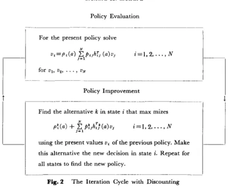
186 Ronald A. Howard Policy Evaluation

For the present policy solve

i=1,2 •...• N

Policy Improvement

- - -

-~---Find the alternative k in state i that max mizes

i=I.2 •...• N

using the present values Vi of the previous policy. Make

this alternative the new decision in state i. Repeat for all states to find the new policy.

Fig. 2 The Iteration Cycle with Discounting

expense of another. An iteration scheme of the same type we described previously accomplishes the job. It is shown in Fig. 2. We select an arbitrary policy and evaluate its present values by using Equation 65. Then we improve the policy by finding the alternative k in each state that maximizes the test quantity

(69)

sing the present values of the original policy. We can see immediately that the test quantity is plausible. When the procedure has been performed for all the states, we have a new policy that we proceed to evaluate, etc. Once more the process terminates when the same policy has been found on two successive iterations.

We shall now prove that the iteration cycle works by following an argument very similar to the one used in the case without discounting. Suppose that policy A has been evaluated and has produced a successor policy B in the policy Improvement procedure. The present values for the policies A and B must each satisfy Equation 65,

(25)

Research in Semi-Markovian Decision Structure6 187 N vf=pf(a)

+

.E

p~hfl(a)lI? j=1 i=I,2, .. . ,N (70) N vj=p1(a)

+

.E

pfjhf/(a)lIj j=1 i=I,2, .. . ,N (71)

If we subtract Equation 71 from Equation 70 we obtain

N N

vf -vt= pf(a) -p1(a)

+

.E

p!jhfl(a)v7 -

.E

ptjhf/(a)vj

j=1 j-1

i=I,2, .. . ,N (72)

Since policy B was produced from policy A as the result of policy improvement,

i=I,2, .. . ,N (73)

We define

ri

equal to the difference between the sides of Inequation 73,

i = 1,2, ...• N (74)

If we now subtract Equation 74 from Equation 72 and write Vi 4=vf-vf, we find

i=I,2, . .. ,N (75)

Equation 75 has the same form as the policy evaluation equations except that the improvements in the test quantity

ri

have replaced the pi(a). Finally if we define column vectors !:!4 and r with components Vi4 and

ri

we can use Equations 67 and

68 to write Equation 75 as

!:!4=Cr (76)

Since we have already shown that the elements of C and

r

are non-negative, the elements of !:!4 must be non-negative. 'The quantity Vi 4 will be greater than zero so

that the present value of starting in state i will be greater under policy B than it was under policy A if it is possible to increase the test quantity in any state

J

that can be reached from state i under policy B. The argument that the iteration process cannot

(26)

stop until it has reached the highest possible present values for each state now follows by analogy with the non-discounting case.

Transient Behavior

In a large number of processes of practical importance we are more interested in the reward the process earns while passing through transient states than we are in the gain of the process. For example, we can often model terminal control systems with different possible trajectories by the kind of model we have been discussing with all states but the terminal state transient. In this type of situation the total reward earned by the process before it enters the recurrent state is the quantity of greatest interest. We can learn about the behavior of such a transient process by writing the policy evaluation equation 37 in the form

N Vt = (qi - g)f i

+

2:

PijVj

j~1

i=I,2, . .. ,N (77)

We interpret this equation by saying that the value of being in state i is equal to the difference between the earning rate and the gain multiplied by the mean waiting time in the state plus the sum of the relative values of all states weighted by the probability of reaching each of them on the next transition. We can clarify the issues involved by assuming that all states but state N are transient and that state N is a trapping state. Since P N N = I, Equation 77 for i = N produces immediately that

g=qN. (78)

If the system were started in state N then the total reward in time t would be simply

qNt. Therefore from Equation 35,vN must be zero, and the other values are uniquely

determined by Equation 77,

i=I,2, ... ,N-I (79)

The first term on the left side of this equation represents the contribution to the ex-pected value of state i due to the present occupancy of this state; the second term represents the expectation of future profit on later transitions. Let ~ be an N-I element column vector with components {(qt-g)ft )} and let P* be the N-I X N-I matrix with elements {pij:i= I, 2, ... , N-I;j= I, 2, ... , N-I}.

(27)

Research in Semi-Markovian Decision Structures 189 Then Equation 79 becomes

(80)

or

!!= [J - P*l-l~ (8I)

The inverse matrix [1-P*]-l always ex:ists for a transient process of the form we have defined. Let

(82) It is a well-known property of Markov ?rocesses that the quantity lii} is the mean number of times the system will occupy state j in an infinite number of transitions. Then

(83)

or

(84)

(85)

Equation 85 says that the value of state i is equal to the sum of the expected earnings from a single occupancy ofstatej, qj 7:j, multiplied by the expected number of times statej will be occupied if the system is started in state i less the gain of the system multi-plied by the expected total time the system will spend in the transient process. The problem of maximizing the expected total reward from starting in a certain transient state in this process is therefore one of selecting the most favorable set of mean numbers of occupancies and earning rates rather than one of selecting the most favorable set of limiting interval transition probabilities and earning rates. We might therefore expect that a slightly different iteration procedure would be advisable.

To establish such a procedure we might examine Equation 77. It suggests that Vi could be maximized by a policy improvement procedure that maximized the test quantity

(28)

with respect to all alternatives k in state i. Note that this test quantity involves not only the relative values of state i under the previous policy, but also the gain of that policy. Let us use the same type of proof we used before to find the properties of this test criterion.

If policy B has been produced from policy A by using this test criterion in a policy improvement, then we can write Equations 49 and 50 for each policy indi-vidually and subtract them. We obtain

i=I,2, .. . ,N (87)

From the properties of the policy improvement,

i=I,2, ... ,N (88)

Let

Ct

equal the difference between the left and right sides of this equation,

N N

Ci

= (qf- gA)rf+

I:

pfjvj- (qt - gAl

rt -

I:

ptjvj

j=! j=!

i=I,2, .. . ,N (89)

Ifwe subtract Equation 89 from Equation 87, we find

i=1,2, .. . ,N (90)

or

i=I,2, ... ,N (91)

If we are dealing with a system in which only state N is recurrent and if the gain of that state is fixed, the gd = 0 and Equation 91 has the same form as Equation 79 with g = O. Therefore by Equation 85.

(29)

Research in Semi-MarkolJian Decision Structures 191 The change in values for each state is given by the sum of the mean number of transi-tions made to each state under the policy multiplied by the increases in the test quan-tity. Since both of the factors are non-negative, all the Vi 4 are non-negative. This

iteration procedure will therefore converge on the policy with the largest values for the same reasons that were discussed in the case with discounting.

We have therefore found a test procedure that will maximize the value of the transient states. We might ask about the effect that using this procedure in all pro-blems would have upon the gain of a process that did not have this transient structure. Equations 91 still apply. We see that they are identical to Equation 58 if

(93) an identity that is easily established. We can therefore write

N

C.

g4 =

L:

M -1

j=l

'i

(94) Equation 94 shows that the increase in gain is not equal to the increases in the test quantities multiplied by the interval transition probabilities of policy B, but rather a division by

ff

is involved. Nevertheless all the arguments about the necessity for the iteration procedure to increase the gain and ultimately to converge on the policy of highest gain apply equally well to this criterion. \Ve do not yet know whether this criterion will increase the gain as quickly as the original criterion, but we do know that it will work and that it will m~ximize the values of a transient process.

Yet there is a disturbing thought-how do we know that the original test quantity, which we shall call the "gain-oriented" criterion, does not miximize the values of a transient process just like the new test quantity, which we shall call the "value-oriented" criterion. Let us check. Equation 58 shows that if gd = 0, then the Vi 4 must satisfy Equation 92 after the mbstitution of

t;;i

from Equation 93; that is,

(95)

We see that the gain-oriented criterion involves not only the mean number oftransi-tions to each state and the increases in te~t quantity but also the mean waiting times in each state. Yet here again all the arguments that show how Equation 92 implies

(30)

a valid iteration procedure still apply. In other words, the gain-oriented criterion will also maximize the values of transient states.

We have now see that both the gain-oriented and value-oriented test quan-tities will accomplish both task we require. The matter of their relative efficiency is still open to question. However, it is easy to show that their efficiencies do differ by considering two examples. The first example is a one state system with three alterna-tives in the state. The system can make only virtual transitions; the alternaalterna-tives specify the earning rates and mean waiting times. The data are

(96)

This trivial system has a trivial solution. Only the gain is involved and from Equation 78 we know that it is just equal to the earning rate of the state. Since alternative 1 produces the highest earning rate, 3, it is clear that this is the alternative on which we want any iteration scheme to converge. Suppose we start with a policy that specifies alternative 3,

1-

= [3]. How will solving the problem using the gain and value-oriented criteria affect the number of iterations required for convergence? We shall begin with the gain-oriented criterion. We already know that for the initial policy

g = 1, Vi = 0. Therefore, the policy improvement procedure of expression 43 be-comes simply Max

qr

We see that this leads immediately to the policy d = [1], and

k

-that the procedure has converged to give a gain g = 3 in one iteration.

Now we shall solve the same problem using the value-oriented criterion of expression 86. We see that it becomes Max (qf~g )fr The test quantities for the

k

three alternatives using the gain of the original policy are then 2, 3, and 0. There-fore, the second alternative is best and we have a policy

r!:

= [2] with gain 2. Now we repeat the policy improvement again and obtain test quantities 1, 0, and ~8.

Now the first alternative is best and we have found the policy!! = 1 with gain 3. Further attempts at improvement lead to the same policy.

We have just seen how in a particular example involving only gains the gain-oriented test quantity was able to find the optimum policy in one less iteration. But is it always better for any problem? No, as we shall now see in a second example with two states. Let state 2 be a trapping state with gain zero and let state 1 be a transient

(31)

Research in Semi-Markovian Decision Structures 193 state that must enter state 2 on its first transition. State I has three alternative ways of going to state 2 described by the three alternatives in display 96. Since the process can earn money only while it occupies state 1 and since the expected amount it will earn doing this is q;'r i, we see that it will eC.rn the most, 8 by following alternative 3. In this problem we find quickly that g =, 0, _V2= 0, Vi = qiT 1 so that solving the

policy evaluation equation is no problem. Let us choose as our intial policy the first alternative in state 1, and indicate this choice simply by

tj

= [1].

Now we have to choose a test quantity. Let us begin this time with the value-oriented criterion of expression 86. Therefore we find immediately that the third alternative is the best and we have converged on the optimum policy

tj

= [3] with a value of 8 in only one iteration.

The gain-oriented criterion of Equation 43 reduces in this problem to the form

For the original policy, Vi = 3 and so we have for the three test quantities 0, 1, and 5/8. Therefore alternative 2 is the best and we change to policy

tj =

[2] for which

Vi = 6. Then we compute the test quantities again and find -3, 0, and 1/4. Now alternative 3 is the best and we have found the optimum policy

tj =

[3] with value

Vt = 8. Of course, further attempts at improvement lead to the same policy.

Now we have seen by example that the value-oriented criterion can save iterations in primarily value maximization problems while the gain-oriented criterion can save iterations in primarily gain maximization problems. "Ve still have not re-solved the question of when each criterion should be used, but we know that the answer has significance. It would seem advisable to consider plans like using the gain-oriented criterion until the gain converged and then switching over to the value-oriented criterion. However, more research on this computational question is needed. Linear Progranuning

Decision problems m semi-Markov processes can be solved by using linear programming just as in the strictly Markovian case; it mayor may not be advan-tageous computation ally to use linear programming algorithms. We shall illustrate how the problems we have discussed can be formulated as linear programs.

(32)

The basic equations for the semi-Markovian reward process without dis-counting are Equations 37,

i=I,2, .. . ,N (97)

By solving these equations for g we can write

i=I,2, .. . ,N (98)

If the gain g and the values Vi are those pertinent to the optimal policy, then for any

possibly non-optimal alternative k in state i,

i=I,2, .. . ,N (99)

N

Let K i be the number of alternatives in state i, and let K =

.E

Ki be the number i=l

of alternatives in all states. Then the gain g must satisfy all the inequalities

i=I,2, ... ,N;

k=I,2, .. . ,Ki (loo)

The gain we seek is the smallest number g that meets these requirements.

We can place this minimization problem in the form of a standard linear program by introducing matrix notation. Since Vs = 0 we can first write Equation

100 as

i=I,2, .. . ,N;

k=I,2, .. . ,Ki (l01)

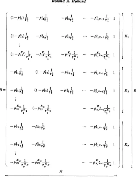
Now we construct a K X N matrix B with elements bij defined by

j=I,2, ... ,N-I

(102)

where

(33)

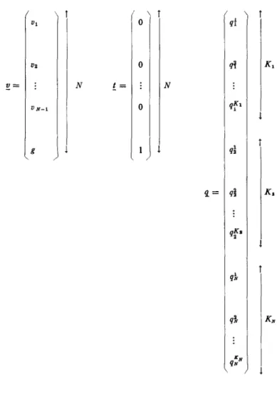
The matrix B is shown in Fig. 3. Then we define two N-element column vectors !:! and !, and one K-element column vector fJ.. These vectors are defined by

i=I,2, .. . ,N-I i=I,2, .. . ,N-I

DN=g

qm(i, k) =q~ (103)

and also shown in Fig. 3.

Now we can write the linear program as Mintll _v

subject to B ~:2

'1

~ unconstrained in sign (104) Here the superscript tT means transpose. This linear program could now be solved by conventional methods.

The dual of this program is interesting in itself. We find immediately from linear programming duality theory that 1he dual is

Max 'ltT1!..

subject to BtT

1!..

=!

1!..:2

0

(105)

The vector

1!.

is a K-element column vec1or. The constraint involving the matrix B is an equality constraint because the primal variables ~ are unconstrained in sign. The dual variables

1!..

are constrained in sign because the constraints involving Bin the primal are inequalities. If we write the detailed equations implied by the matrix formulation 105, we find that the dual variables are the different possible limiting interval transition probabilities for the semi-Markov process. Formulation 105 is therefore a method for maximizing the right-hand side of Equation 41.

The decision process with discounting is also susceptible to linear programm-ing. In this case the basic equations are Equations 65

(34)

196 _{ROllald A. Howard}

(l-pb)

h

1 I

-P,'H

-P'31

¥"!

I - P"N-I 1

H

I I

-Pi

2

J

2

2 I I

K,

(l -

P~l)f1 ~,

- P'3f1

-Pi,N-l

f1

K I pK,_I_

KI

I K, I

(l-Pu

l₎

-- 12 _KI _-P13

_rKI

- PI,N-IrK I

rKI 1 ~l 1 1 1 I

(l-p~2)h

-pkA 1 I

-P21fj

_~2

-P2,N-Ifj

B=

_- p' _21f]I

_(l-Pi2)h

2 I -P23¥l _ 2

P2,N- Ifi

.l

K,

K KZ I K2 I Kz I -Pu :K (-P22

fK,

-P2,N-I rK2 ~2 I ₂ 2 1 I -PN1il - p' N2fJ I -PN,N-IfJ 1 I 2 I

-PNl¥A -PN2¥A 2 I _ 2 _PN,N-IrA

.l

KN

KN I KN I KN I

-PNI rKN -PN2 rKN -PN,N-I

r KN

N N N

N

(35)

v=

Research in Semi-Markovian Decision Structures

Vz N t= VN-l g

o

N

o

qf

qKl 1 q} qK. 2

Fig. 3 Matrix Definitions for Linear Programming Formulation

(36)

We now want to maximize the present values Vi. By the same argument that we followed before we know that the v;'s we seek are the smallest v;'s satisfying.

i=i,2, .. . ,N (106)

cll

(108)

We construct the matrix formulation by defining a matrix D whose elements are

j=I,2, ... ,N (109)

We also define two N-element vectors ~ and ~ and one K-element vector eCa) with elements

Vi=Vi, i=I,2, . .. ,N; s;=I, i=I,2, .. . ,N

(110)

These new definitions may be easily visualized in the format of Fig. 3. Since maxi-mizing the sum of the present values is equivalent to maximaxi-mizing each of them in-dividually in our problem, the linear program is

Min SIT V

subject to D !!.ze(a)

~ unconstrained in sign (Ill)

Once more the dual of this problem is significant. Let E be a K-element column vector. Then the dual of this linear program is

Max etr(a) q subject to Dtr q = ~

(112)

The detailed equations implied by formulation 112 show that the components of E are just the discounted number of times we expected each state to be occupied in an infinite number of transitions. Therefore this formulation is equivalent to maximizing

(37)

Research in Semi-Markovian Decision Structures 199 the set of present values as expressed by Equation 67. Once more we see that the dual formulation has an important interpretation.

Now that we have seen a linear programming formulation of the problems we have been discussing it is worth mentioning that the dual is computationally much more convenient than the primal. The primal has 2N+K variables because the constraints are inequalities and the variables are unconstrained in sign; it has K equations. The dual has K variables and N equations. Since K is usually much larger than N, we find it more convenient to solve the dual formulation in almost all cases. Sununary

Decision models of the type we have discussed are interesting mathematical developments, but they are useful in practical problems only if we can supply them with necessary data. Consequently, we are investigating schemes for deriving this data from both experience and experiment. We are also investigating how to solve the decision process when the data are uncertain. Although the practicality of these methods will be considerably enhanced by the completion of this research, the model as it stands continues to have important application in several areas of management systems.

REFERENCES

1. Howard, R. A., Dynamic Programmtng and Markov Processes, Technology Press-Wiley, Cambridge, 1960.

2. Levy, Paul, "Systems Semi-Markovian a au plus une infinite denombrable d'etats pos-sibles, "Proc. Int. Congr. Math., Amsterdam, Vol. 2 (1954), p. 294. "Processes Semi-Markovian," ibid., Vo!. 3 (1954), pp. 416-426.

3. Smith, W. L., "Regenerative stochastic processes, "Proc. Roy. Soc. (London), Ser. A, Vol. 232 (1955), pp. 6-31 (cf. the abstract of this paper in Proc. Int. Congr. Math., Amsterdam, Vol. 2 (1954), pp. 304-305.

4. Smith, W. L., "Renewal theory and its )'amifications,"

J.

Roy. Stat. Soc., Ser. B, Vol. 20 (1958), pp. 243-302.

5. Pyke, R., "Markov Renewal Processes with Finitely Many States," Annals, Math. Stati., 32: 1243-59.

6. Howard, R. A., "Semi-Markovian Dectsion Processes," Proceedings of the 34th Session of the International Stati~tical Institute, Ottawa, Canada August 21-29,1963.