A Sequencing Model with an Application to Speed Class Sequencing in Air Traffic Control

Operations Research

Society of Japan

VOLUME 17 March J974 NUMBER 1

A SEQUENCING MODEL

WITH

AN APPLICATION

TO SPEED CLASS SEQUENCING IN

AIR TRAFFIC CONTROL

YUKIO TAKAHASHI Tokyo Institute of Technology

(Received June 12, 1972)

Abstr:act

Servicing systems with two or more types of customers are considered. In such a system, a server may suffer a loss in efficiency if he switches service from one type to another of customers, because he may require some transfer time besides net service time. So, if the order of service is changed by a sequencing policy, the total time required to serve all customers, say N customers, may be decreased and the efficiency may be increased. In this paper the amount of such improvement of the efficiency of a system is evaluated under some idealized conditions.

We first deal with speed class sequencing in air traffic control and set up a model with two types of customers. For the model we obtain an optimal sequencing policy under a restriction which assures that no customer has a long wait, and calculate the mean service time under the policy. We also study a system with three types of

customers. For the case we obtain the mean service time under a policy using a Markov chain and graph the results'of the calculation.

1. Introduction

In order to relieve the air traffic congestion at a terminal, se· quencing of landing aircraft by their speeds has been proposed and analyzed with computer simulations by many authors in private papers. Here we shall study theoretically how the efficiency or the landing capacity can be increased by adopting speed class sequencing under some idealized conditions.

We set up a model in Section 3, while in Section 2 speed class sequencing in air traffic control is briefly explained and also the plan of setting up the model is shown from the point of view of speed class sequencing. The model is so simple that it can be applied to many other queueing problems of the following type: There are two (or more) types of customers. A server serves customers one by one, and besides net service time he requires some transfer time for switch· ing service from one type to another. Then, compared with the first·come first·served policy, how can we increase the efficiency or the capacity of the system in a busy period by reordering (sequencing) the customers?

Problems of this type could be analyzed using the theory of multi· queues or the theory of priority queues. However these theories are very difficult and have been solved only in the simplest cases. Although our model is very idealized, it has many applications because of its simplicity. For example, it might be applied to some queueing models in computer systems or to some job·shop scheduling models.

2. The Speed Class Sequencing

We shall start with a variant of the model by A. Blumstein [1] for the analysis of the landing capacity. We consider a single runway which is used for landings only. Aircraft pass through an imaginary

gate in space and follow a common glide path to the runway. To schedule the passing times through the gate, two conditions for security must be satisfied:

( a) When an aircraft passes through the gate, the distance from the next aircraft should be greater than d (some fixed distance). ( b ) There can be only one aircraft on the runway at a time. We wish to schedule the passing times through the gate so that the time intervals between successive passing times are as short as pos-sible. It is convenient to define that the service time of an aircraft is the time interval between the passing times through the gate of it and of the preceding one. Then the service time of an aircraft depends not only on its own speed but also on the speed of the preceding one. Let the lengths of the glide path and the runway be m and [, respectively (see Fig. 1). Suppose that an aircraft with speed Vl follows

one with speed Vo. (We assume that the speed of each aircraft is constant in the area under consideration around the terminal. Mod-ifications to the real situation would be obvious.) Let to be the scheduled passing time of the preceding aircraft through the gate.

r.te Runwav.

~ _____________ "~"~ _____ .~r.~li'~le~p~at~h ______ i=====~

~---d~---~~---Time

Then the aircraft goes out the runway at to+(m+l)/vo. If the follow-ing aircraft passes the gate at tl, it reaches the runway at tl +m/vl. Hence by the condition (a), tl must be greater than to+d/Vl, and by the condition (b) tl +m/vl must be greater than to+(m+l)/vo. For the shortest service time of the following aircraft, we should schedule its passing time through the gate as

( 1 ) tl=tO+ max (d/Vl, (m+l)/vo-m/vl), and then the shortest service time of it is given by

(2) 51=tl-tO= max (d/Vl, (m+l)/vO-m/vl).

We may regard the service time SI in (2) as the sum of the net service time d/Vl and the transfer time 51-d/Vl. Since ordinarily d>t because of the inaccuracy of the estimation of the position of an craft, non· zero transfer time is required only when the following air-craft is slower than the preceding one. Hence in order to increase the efficiency or the landing capacity, it is necessary to decrease the rate of switches from fast aircraft to slow ones by sequencing. This is the basic idea of speed class sequencing in air traffic control.

In order to decrease the rate of switches from fast aircraft to slow ones, we should sequence aircraft so that as many aircraft as possible with the same speed land continuously. But if too many aircraft with a specific speed land continuously, there may be aircraft with faster or slower speed having long waits, and this is inadmissible in practical situations. Hence we should seek an optimal sequencing policy in the set of policies satisfying some restrictions which assure that no air-craft waits too long. This will be reflected on the four kinds of restrictions in our model in Section 3.

We shall restrict our concern to the case where there are always sufficiently many aircraft waiting for landing, because it does not matter if few aircraft are waiting. Then, together with the restric-tions on the sequencing policy, we may treat our model supposing that all the aircraft under consideration have already reached the area around the terminal and are waiting for services at the beginning of

the first service.

In practice, landing aircraft have various speeds. However in speed class sequencing, we have to schedule the passing times through the gate in advance. We have to predict their speeds from the informations on the types of them and we have to sequence them subject to the predictions. So we might as well classify aircraft by their types, and as the simplest case, we shall consider two aircraft types (e.g., jet planes and turbo·prop planes).

3. A Sequencing Model with Two Types of Customers

Now we shall set up our modeL We consider a servicing system with a single server. There are two types of customers denoted by type 0 and type 1. Each customer of type i (i=O, 1) demands net service time of length Si. When the types of two consecutive cus-tomers are different, the server spends some transfer time besides the service times required by the customers. We assume that the server spends transfer time of length Ti when the service switches from type

(I-i) to type i. Suppose that N customers have already arrived and

are waiting for services in a queue in the order of arrivals. We are interested in the total time required to serve all the N customers under a sequencing policy. (We can treat models with looser assump-tions than this model. See Remark 1 at the end of this paper.)

We will represent the types of the N customers in the queue by a binary sequence (el, e2, ... , eN) where en is equal to 0 or 1 according to the type of the nth customer. A" sequencing policy" or simply a "policy" is a permutation

(1

2 . . .

N)

which determines the

ml m~ ... mN

order of services. Under the policy, the nth customer is served in

the mnth service. The original binary sequence which represents the

types of customers in the queue, is transformed to a new binary sequence (e;, e;, ... , e~v) which represents the types of customers in the order of services where e~n=en. W"e shall call the original sequence

e;, ... , e~-) the reordered sequence.

We shall use the term "the service time of a customer" as the sum of the net service time required by it and the transfer time preceding it. Then the service time of the nth customer is given by

(3 ) if e;'=e;'_l

if e;'*e:,.-l

w here m

=

mn . So the total time required to serve all the N customers under the policy is

N

(4)

2:

S(n)=NoSo+NISI+MoTo+MITI

n=l

where Ni (i=O, 1) is the number of m's such that e;.=i (i~m~N), i.e., the number of customers of type i, and Mi (i=O, 1) is the number of m's such that e;.=i and e;'_l=l-i (2~m~N), i.e., the number of switches of service from type 1-i to type i. In order to discuss the asymptotic behavior as N to infinity, it is convenient to introduce the (arithmetic) mean service time

( 5)

We shall call PN= No/ N the ratio of customers of type

°

(in the N customers) and qN=NJ/N the ratio of customers of type 1. And we shall call aN=Mo/N the ratio of 1-0 switches (in the N services) and

f3N=MI/N the ratio of 0-1 switches.

We note that the ratios of customers of type 0 and type 1 are invariant under any policy. So, the mean service time is determined by the ratios of 1-0 and 0-1 switches. The smaller the ratios of 1-0 and 0-1 switches, the smaller the mean service time. So in order to minimize the mean service time, if To> T I, we might adopt a policy under which all customers of type 0 are served first and then customers _, of type 1 are served. However in most practical applications, all policies cannot be adopted, but available policies are ones under each

of which mn is not so distant from n for each n. So we should con-sider that available policies are ones which satisfy a certain restriction on mn, and here we shall study the following four kinds of restric-tions. (For other restrictions, see Remark 2.)

Ro: mn=n (i.e., the first-come first-served policy)

RI: m,,<mn+kH for all nand i (>0).

R2: Imn-nl~k

Ra: mn~n+k

for all n. for all n.

In the above restrictions, k expresses the allowance limit of exchanges, and when k =0, RI, R2 and Ra coincide with Ro. Let Pi (i=0, 1,2,3) be the set of all policies satisfying the restriction Ri. Then for fixed k, clearly PiePj if i<j.

Now we shall consider an optimization problem of the sequencing. For each arrival sequence, we say that a policy is optimal in Pi if it minimizes the mean service time

SN.

Problem. Find an optimal policy in Pi (i=1, 2, 3).

The answer to this problem is given in the next section. 4. An Optimal Policy

Now we seek an optimal policy in each Pi. We can show that the following rule leads us to an optimal policy. By the rule we can decide which customer should be served next. We are convenient to use the terms concerning the queue in the servicing system. We assume that customers in the queue are in the order of arrivals. Rule I: Serve the first customer of the same type as one being served

in the queue, unless it conflicts with the restriction Ri. If it con-flicts with Ri or if there is no customer of the same type as one

being served in the queue, then serve the customer at the top of the queue.

In order to determine a policy by this rule, we must choose a customer to be served at the outset. Two special cases are considered.

Input sequence Reordered sequence ~ 0 0 1 ,0 1 11 M,,~9 .11,.··10 /?,,,,,><,,,.;>-~,

'>-:"

.... "

"

~ "-I 0 0 0 0 0 1 1 1 M" ~. 2 M, = 3 o '~

"

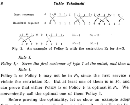
, 1 1

Fig. 2. An example of Policy 10 with the restriction RI for k =3.

Rule l.

Policy I,: Serve the first customer of type 1 at the outset, and then adopt

Rule l.

Policy 10 or Policy 11 may not be in Pi, since the first service may violate the restriction Ri. But at least one of them is in Pi, and we can prove that either Policy 10 or Policy 11 is optimal in Pi. We will conveniently call the optimal one of them Policy I.

Before proving the optimality, let us show an example adopting Policy 10 to a sequence under the restriction RI. (See Fig. 2.) In this case Rule I can be rephrased as follows.

Rephrased Form of Rule I under the Restriction R ,:

If the server is servicing a customer of type 0 and if the customer

at the top of the queue is of type 1, then before servicing the top of the

queue, let the server serve customers of type 0 in the first (k

+

1) customers

of the queue. And then let him serve customers of type 1 until a customer of type 0 comes to the top of the queue. In the contrary case, do the same way exchanging the roles of 0 and 1.

Hence in the example the mean service time

525

is decreased from

_{S25=25So+2SS1+25To+25Tl}

- 12 13 9 10 (under FCFS)

to

_{S25=25So+2SS1+25To+25Tl}

- 12 13 2 3 (under Policy 10)

The Proof of the Optimality of Policy I

Now we shall prove the optimality of Policy I. Here we prove it under the restriction RI, and for other restrictions we can prove it

in the same line. We prove it in two steps.

Lemma. There exists an optimal policy in the class Pi (c Pt) of policies

satisfying the condition that m ..

<

mn , for each pair of nand n' such that

n<n' and S"=Sn" (In other words, it is sufficient to seek an optimal

policy in the' class Pi of policies under which the first-come first-served rule is adopted for the customers of the same type.)

Proof. Let the input sequence be (SI, S2, S3, " ' , SN), and under a policy

in Pi let the nth customer be served in the m"th service. Suppose that there is a pair of integers nand n' (n<n'), such that S"=Sn"

m,,=x, mn,=y and x>y. By the definition of RI

(6) x <m,,+1<+i

for all positive

i.

Then, since y <:r,

(7) y<m,,+k+i

for all positive i, and since n<n',

(8) x<m,"+k+i

for all positive

i.

Hence there is another policy in Pt which transforms the input sequence in the same manner as the original policy except that m,,=y and m",=x. Since S"=S~" the ratios of 1-0 switches and 0-1 switches are the same in both policies, and this shows that an optimal policy is in the class Pt.

Theorem. Either Policy 10 or Policy Tt is optimal in Pt.

Proof. Let us consider an optimal policy in Pt and name it Policy

n.

Suppose that (m-I) customers have been served under Policy II and that s:"_,=O (i.e., a customer of type 0 has just been served). If the

nith customer (i=O, 1) is the first customer of type i in the queue,

then under Policy

n,

either the no th or the 111 th customer is served next. Three cases can be considered. In order to satisfy the restric-tion RI,

( i) the noth customer must be served next. (ii) the nlth customer must be served next.

In the first two cases we have no alternative, and we can consider that Policy II adopts Rule I in this step. In the third case, if m"o=

m (i.e., the noth customer is served next), Policy II adopts Rule I in

this step. If m"l = m, we can prove that there exists another optimal policy which adopts Rule I in this step.

Suppose that we are in the third case and that m"l=m under Policy H. Let M~'(j, j') be the number of 1-0 switches from the jth service to the j'th service. Then the number of 1-0 switches in the N services is given by

(9) M:'=M:'(l, N)=M:'(l, m-1HM~'(m-1, mHM:'(m, N)

=M~'(l, m-1HO+M~'(m, N).

We define Policy HI as follows. Under Policy IH, the server serves (m-I) customers in the same manner as Policy H, and then serves the noth and the tllth customers in this order. And he serves the remaining (N-m-1) customers in the queue in the same order as Policy Il except for the noth customer. Then Policy III adopts Rule I at the mth service, and we can easily prove that Policy III is in Pt. The number of 1-0 switches under Policy III is given by

(10) M:"=M:"(l, N)=M:"(l, m-1HM:"(m-1, m+1)

+M:"(m+1, N)

=M:"(l, m-1HO+M:I1(m+1, N).

Now we shall compare M:'(m, N) with M:"(m+1, N). The segment from the (m+ l)st service to the Nth one of the reordered sequence under Policy III is the same as the segment from the mth service to the Nth one of the reordered sequence under Policy Il except that a type 0 service has been gone out. Hence

(11) M:'(m, N)~M:"(m+1, N).

Since M:'(l, m-1)=M:II(I, m-I), we have

(12) M~'~M:"

by (9), (10) and (11).

in a similar way. Hence we have (13) S~;;;S~lI.

It follows that Policy III is also optimal, since Policy 11 is optimal. Using the above result, we can prove by the mathematical induc-tion on m that there exists an optimal policy in

Pt

which adopts Rule I in each step. Such an optimal policy is either Policy

10

or Policy 11, and this proves the theorem.

5. The Limiting Mean Service Time under an Optimal Policy

Now we shall investigate how much we can decrease the mean service time by adopting the sequencing. For the purpose, we are convenient to assume that the input sequence is a Bernoulli sequence with probabilities p of type 0 and q of type 1 (p+q=I). Namely we assume that el, e2, " ' , eN are mutually independent random variables with the common distribution P(ei==O)=P and P(ei=I)=q. Then by the law of large numbers, the ratios PN and qN of customers of type

o

and of type 1 converges to P and q with probability one as N->oo. By the renewal theorem, we can prove that the ratio aN of 1-0 switches under Policy I converges to a limit a with probability one as N->oo. The ratio {3N of 0-1 switches under Policy I also converges to the

Table 1. The limiting ratio- a of 1-0 switches under an optimal policy in Pi.

Restriction Ro RI Rz Rs a pq pq/(1+2kpq) pq/(1+2pqE(Zlc» (*) pq/l1+k)

(*) Zlc is a random variable having the following distribution.

{( t-l )(P!"It-Ic+pt-Icqlc) if k<t5:.2k-l

P(ZIc=t) = k-l = - ,

Table 2. E(Zk) for small k. o 0 1 1 2 2(1+pq) 3 3(1+pq+2p2q2) 4 4(1+pq+6p2q2+5p3q3)

same limit a with probability one as N---->co, since always

I

Mo-Mll~1. Hence we can write the limiting mean service time as

(14) S=pSO+qSl +a(To+ Tl).

Table 1 shows the limit a of 1-0 switches under an optimal policy in Pi. In the remaining of this section, we shall prove it. In the sub-sequent discussions, we sometimes argue as if N is infinity and omit the word "limiting".

( i) The case under the restriction R,

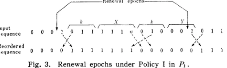
In this case Rule I can be rephrased as in Section 4. Hence, considering the input sequence as a discrete time stochastic process, we may take the time as a renewal epoch when a customer of type 1 comes to the top of the queue during a continuous service of cus-tomers of type 0 (see Fig. 3).

Then the length of a cycle from a renewal epoch to the next renewal epoch is given by

(15) L=2k+X+ Y

where X and Y are random variables representing the number of

Input

sequence

Reordered

sequence

Fig. 3. Renewal epochs under Policy I in Pt.

1 I

customers required up to and including the first arrival of a customer of type 0 and of type 1, respectively, in a Bernoulli sequence. Since X and Y have geometric distributions, the mean cycle length is given by

(16) E(L)=2k+-+-=-(1+2kpq) . 1 1 1 p q pq

In each cycle, just one 1-0 switch occurs. Hence by the renewal theorem, the limiting ratio a of 1-0 switches exists with probability one and is given by

(17) a=I/E(L)=pq/(1+2kpl]).

(ii) The case under the restriction R2

We may take similar renewal epochs as in (i) (see Fig. 4). In this case a cycle consists of four mutually independent random variables Wl, X, W2 and Y. Customers of type 0 in W1 are served before the

customer of type 1 who is the last one in preceding Y, and customers of type 1 in W2 are served before the customer of type 0 who is the

last one in X. X and Y have the same distributions as in (i). Wi

(i=l, 2) is the number of customers required in a Bernoulli sequence

until at least k customers of type i arrive. Then we can easily show that Wi has the distribution given under Table 1. Hence it follows

that the mean cycle length

(18) E(L)=E(WIHE(XHE(W2HE(Y)

sequence

1 1

=2E(ZkH-+- , p q

Jnput sequence Reordered sequence _ _ _ _ _ Renewal epochs----~

.. r;,

~o

";;-;--;'OO! .cO" •

~

'-:J",

><>:/

>~~-:-:.::::-:.:,

__ \-\-\-

0

J,),~,>\:

__

,: .... /~.: ' ... ""... ...- ,.,.- ;.-.-....,... " ,," I " ... ~:' 0 0 0 0 0 1 1 1 1 1 1 1 1 0 0 0 0 0 0 0 0 0 0

Fig. 5. Renewal epochs under Policy I in Pa•

and that the limiting ratio of 1-0 switches (19) a=pq/(1+2pqE(Z,,)).

(iii) The case under the restriction Ra

We use similar renewal epochs as in (i), too (see Fig. 5). In this case a cycle consists of four mutually independent random variables U, X, V and Y. Customers of type 0 in U are served before the customer of type 1 who is the last one in preceding Y, and customers of type 1 in V are served before the customer of type 0 who is the last one in X. X and Y have the same distributions as in (i). U is the number of customers required in a Bernoulli sequence up to and including the kth arrival of type 0, and V is a similar one for type 1. Then U and V have negative binomial distributions. Hence it follows that the mean cycle length

(20) E(L)=E(

UH

E(XH E(

VH

E( Y)

k 1 k 1 k+l

=-+-+-+-=--,

_{p p q q pq}

and that the limiting ratio of 1-0 switches

(21) a=pq/(I+k).

6. Comparison between Policy I under the Three Restrictions We have considered three restrictions RI, R2 and Ra, and obtained an optimal policy in each case. However the optimality discussed here reflects only the efficiency of the system. In general, a measure for goodness of a policy may contain more factors. In speed class

sequencing, the measure might have factors such as the efficiency of the runway, the simplicity of the control, the mean number of aircraft which go ahead of a certain aircraft, and so on. Hence we should decide the measure taking account of the pattern of the landing air-craft, the ability of the control system, the security in the sequencing, feelings of people for the delays caused by the sequencing, and so on. If the measure is determined, we might be to seek an optimal policy with respect to the measure. However, such an approach is sometimes difficult. There is another approach in which we shall be engaged. We choose several policies and study their properties. And in the application, we adopt one of them which is best of all with respect to the measure. So we might as well study properties of Policy I under each restrictions.

Here we consider only the mean number f1. of aircraft which go

I'

2.0

1.8

,3

i (Nurrbers attached to nodes

1.6 i repl"~sent the yalues of h)

8i 1.4

i

7 \2 1.2

\

6 _\ 4 _\ 1.0 _,

\

5 0.8 \ 3 4 \1 \ 0.6 _, \

.,

3 \ 2 '. '\ \fu 0.4 _{fu '" R, \} ,,~ \ 0.2 2 ~I \

~

1 "-:~ la 0 0 . 05 .10 .15 .20 .25

Fig. 6. The mean number p. of airerafts which go ahead of a certain aircraft and the ratio a of 0-1 switches under Policy I (p=0.7, q=0.3).

ahead of a certain aircraft. p. can be also considered as the mean delay E[m,,-n] + caused by the sequencing, or as a half of the mean absolute departure El m,,-n

I

of m", from n, since E(mn)=n. Table 3 shows the result of the calculation of p., and Fig. 6 shows a numerical example for p=0.7 and q=0.3. There may be an optimal policy in Pi which has smaller p. than Policy I. For example, if the input sequence is (0, 0, ... , 0, 1, 0, ... , 0), then for each restriction Ri, p.= kiN under Policy I, but p.=0 under the first-come first-served policy which is also optimal for the sequence. Hence we might be to seek an optimal policy in Pi which minimize p.. Unfortunately, we have not yet find such an optimal policy. However under such a policy, prob-ably we cannot decide the servicing order one by one, and so the control is more complicated than Policy I.

In order to prove the results in Table 3, we return to Section 5. For the case under the restriction RI, we consider a cycle in Fig. 3. Aircraft of type 1, which arrive after an aircraft of type 0 and are served before it, are in the third interval denoted by k. If the ith aircraft in the interval is of type 0, the mean number of aircraft of type 1 which go ahead of it is (k-i)q. And for the last aircraft in the second interval denoted by X, the mean number of aircraft of type 1 which go ahead of it is kq. These are the only aircraft of type 0 for which m,,>n. We can obtain similar results for aircraft of type 1 for which m,,>n. Hence the mean number p. of aircraft which go ahead of a certain aircraft is given by

Table 3. The mean number p. of aircraft which go ahead of a certain aircraft under Policy I.

Restriction p.

kpq(1+(k -l)pq) 1(1 +2kpq) pq {(k +3/2)E(Z,,)- k} 1(1 +2kpqE(Z,,» 2kpq/(k+1)+kI2

pq

[I:

I:

]

(22) p= 1+2kpq ~(k-i)pq+kq+ ~(k-i)qp+kp

kpq

1+2kpq [1+(k-1)pq].

This proves the result in Table 3 for RI. For the restrictions R2 and Rs, corresponding results are proved in a similar way, and the proofs are not presented here. We only notice that it is recommended to calculate E[n-m,,]+ instead of E[m,,-n]+ in the proofs.

7. An Example with Three Customer Types

If the number of types of customers are more than two, in order to calculate the limiting ratios of switches of the type of service, the renewal theoretical technique used in the last section cannot be adopted, but we can use a Markov chain technique. As an example we con-sider a servicing system with three types of customers under the restriction RI (defined in Section 3). In this case we can hardly find an optimal policy, because if we try to get an optimal policy the selection of the next served customer depends not only on the type of the customer being served, but al.so on the whole sequence. This reflects an essential difference between the cases of two types of customers and of three or more types of customers. Hence here we are content with a policy adopting Rule I. We study with

Policy 1': Serve the first customer at the outset, and then adopt Rule I. Since our aim is to obtain the limiting ratios of switches of the type of service, we can take an infinite sequence (el, e2, ea, ... ) as the input sequence. We assume that it is a sequence of mutually inde-pendent random variables e" (n= 1, 2, 3, ... ) with a common distribution

(23) P(e,,=a)=p, P(e,,=b)==q and P(e,,=c)=r (p-t-·q+r=l).

In order to calculate the limiting ratios of switches of the type of service, we must define a Markov chain. However it is instructive

to study an example of services under Policy I' before we define the Markov chain.

Let us consider an example for k=3 in Fig. 7. Customer 1 is served first. Then Customer 2 comes to the top of the queue, but he is of different type with Customer 1. Hence we seek customers of type a among Customers 3-5 who can be served before Customer 2 without conflict with the restriction RI. We find that Customer 4 is of type a. Then we decide that Customer 4 is served next and that Customer 2 is served after him. Thus the server serves these customers in the order: 1,4,2. When Customer 2 is served, Customer 3 is at the top of the queue. Since he is of different type with Customer 2, we seek customers of type b among Customers 4-6 who can be served before Customer 3 without conflict with the restriction RI. (Customer 4 has already been served and he is not in the queue. But in order to clarify the range for search, it is convenient to treat as if he were in the queue.) However we can find no customer of type b, and so we decide that Customer 3 is served next. When Customer 3 is served, Customer 5 is at the top of the queue. Since he is of the same type as Customer 3, he is served immediately after Customer 3. The same situations arise for Customers 6 and 7. When Customer 7 is served, Customer 8 is at the top of the queue. Since he is of different type with Customer 7, we seek customers of type e among Customers 9-11. Since Customer 9 is of type e, we decide that he is served immediately after Customer 7, and then Customer

Customer Input sequence States Reordered sequence Customer 1 2 3 4 5 6 7 8 9 10 11 12 13 14 15 16 17 18 19 20 a b c a c e c a e b b c a b b a c e a a ~~~771101237~11o123~ ~ 0 1 2 3

*

~ ~ ~ 0 1 2 3

* *

~ ~ ~ ~ ~ tt~~~~~~~~~~~~~~~~~t a a b e e c c c a a b b b b e e c a a a 1 4 2 3 5 6 7 9 8 13 10 11 14 15 12 17 18 16 19 20

8 is served.

Now we define a Markov chain which represents the transitions of the type of service. There are ma.ny such Markov chains, but the one defined below has a fairly small number of states.

Since we are interested in the limiting ratios of switches of the type of service, we need not know exactly when a switch of the type of service occurs, but need only know the fact that it occurs at some time. Hence we define the Markov chain so that it can indicate only the occurrences of switches of the type of service. A switch of the type of' service occurs if and only if a customer is not served im-mediately after a customer of the same type. And in such a case, he comes to the top of the queue when a customer of different type is served. Hence we can consider that these three contents represent the same situation. It is convenient to explain the definition of the Markov chain by tracing the transitions in the example in Fig. 7.

We consider that a transition of the Markov chain occurs when a service has finished. The state of the Markov chain at time n (n=

1, 2, 3, ... ) is denoted by a triple (Sa(n), sb(n), Seen)), and each entry

si(n) (i=a, b, c) of it varies over a set

ifJ,

0,1,2, ... , k,

*.

In Figures 7 and 8, we write the state in the form of a column vector for the convenience of printing.

In the example in Fig. 7, the Markov chain starts with the state

(*,

ifJ,

ifJ)· Generally, that si(n)=ifJ (i==a, b, c; n=l, 2, 3, ... ) represents such a situation that Customer n is not of type i and even if he is of type i, he will not be served immediately after a customer of type

z. And that si(n)=* represents such a situation that if Customer n

is of type i, then he will be served immediately after a customer of type

i.

In this case Customer 1 is the first customer and there is no customer who is served before him. However it is convenient to consider that there is a customer (say, Customer 0) of the same type as his and that he is served immediately after the customer. Hence here we set s",(l)=*.

Customer 2 is of type b but since so(l)=.p he will not be served immediately after a customer of type b. We represent this situation by setting so(2)=0. Generally that si(n)=O (i=a, b, c; n= 1, 2, 3, ... ) represents such a situation that Customer n is of type

i

and he will not be served immediately after a customer of type i. Hence if si(n) =0, then Customer n will come to the top of the queue when a customer of different type is served. Returning to the example, so(2) remains at

.p

and s,,(2) also remains at

*,

because if Customer 2 is of type a, he will be served immediately after Customer 1. Hence the state of the Markov chain at time 2 is (*,0, .p).

When a customer of different type with one being served comes to the top of the queue, we must seek customers of the same type as one being served. In this case we must seek customers of type a among Customers 3-5. In order to indicate these customers among whom we seek customers of type a, we set so(3)=1, so(4)=2 and so(5) =3. We can indicate that we seek customers

of type a

by setting s,,(3)=s,,(4)=s,,(5)=* (see the meaning of

*

stated above). Generally if si(n)=O (i=a, b, c; n=l, 2, 3, ... ), then in order to indicate the range for search, we set si(n+1)=1, si(n+2)=2, ... , si(n+k)=k. Of course, in the case, customers of type i among Customers (n+1)-(n+k) are served successively after Customer n. Hence besides the above mean-ing, that si(n+ j)= j (j=1, 2, ... , k) also represents the same situation as the case of

*.

For the state at time 3, we have already shown that s,,(3)=* and so(3)=1. Since Customer 3 is of type c and so(2)=.p, so(3)=0 by the same reason as Customer 2. Hence the state at time 3 is (*, 1,0).

When Customer 3 comes to the top of the queue, we seek cus-tomers of type b among Cuscus-tomers 4-6. In order to indicate these customers, we set so(4)=1, so(5)=2 and so(6)=3. And in order to indi-cate that we seek customers

of type

b, we set so(6)=* since we have already set so(4)=2 and so(5)=3. Thus the states of the Markov chain from time 1 to time 5 are found to be as shown in Fig. 7.

For the state at time 6, sb(6) and so(6) have been set to

*

and 3, respectively. The state at time 5 in which s,,(5)=* and sb(5)=3 im-plies that customers of type a among Customers 3-5 are served before Customer 2 but Customer 6 cannot be served before Customer 2. Hence even if Customer 6 is of type a, he will not be served im-mediately after a customer of type a. In this case Customer 6 is not of type a and so s,,(6)=rp. Thus the state at time 6 is (rp, *, 3). Generally if si(n-1)=* (i=a, b, e; n=2, 3, 4, ... ) and if si,(n-1)=k for some i' (if =a, b, e and *i), then si(n)=O when Customer n is of type i and si(n)=rp when Customer n is not of type i.

At time 7, sb(7) is <p by the same reason as stated above, and

s,,(7) remains at rjJ since Customer 7 is not of type a. Since so(6)=3

and Customer 7 is of type e, he wit be served immediately after a customer of type e. So so(7)=*. Thus the state at time 7 is

(<ft, <ft,

*).

Generally if si(n-1)=k (i=a, b, e; 11=2,3,4, ... ), then si(n)=*. At time 8, since Customer 8 is of type a, s,,(8)=0 and sb(8) and

so(8) remain at rjJ and * respectively. Hence the state at time 8 is

(0, rp, *). We can proceed in like manner.

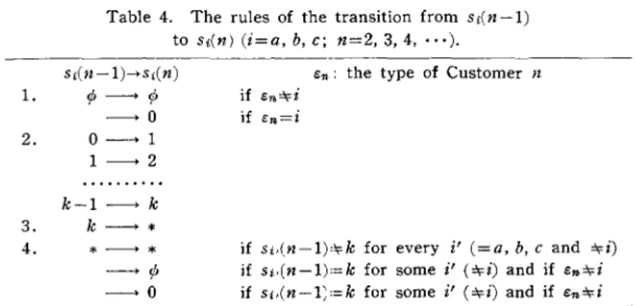
We can tabulate the rules of the transition from si(n-1) to si(n)

(i=a, b, e; n=2, 3, 4, ... ) as in Table 4 in which En represents the

type of Customer n.

Table 4. The rules of the transition from si(n-l)

to si(n) (i=a, b, c; n=2, 3, 4, ... ). si(n-l)->si(n) 1. <P ---> <P 2. ---> 0 0--->1 1 ---> 2 k - l ----> k 3 • k --->

*

4. _{* ---->}

_*

if En"ri if en=i

En: the type of Customer I!

if si,(n-l),,,,k for every if (=a, b, c and "ri)

jf si,(n-l),=k for some if ("ri) and if E .. "ri

This Markov chain can indicate the occurrence of a switch of the type of service. If si(n)=O (n= 1, 2, 3, ... ) for some i (=a, b, c), then Customer n will not be served immediately after a customer of the same type. Hence we can know the occurrences of switches of the type of service by the appearances of O. Further, in order to know the appearances of 0, it is convenient to see the transitions of

*.

Because, each 0 is followed by an * in the same entry of the state just after k epoches, and from one such * to the next such *, the same entry of each state as the former

*

is filled with

*.

The set of possible states (Sa, Sb, Se) (Sa, Sb, Se=</>, 0, 1, 2, . - -, k, *)

of the Markov chain can be divided into six classes [ab], [ae], [ba],

[be], [eaJ and [ebJ. For the purpose, we introduce an order -< into the

set of the symbols as follows: </>-<0-<1-<2-<··

·-<k-<*.

The class [ijJ (i, j =a, b, e; i* j) consists of states (Sa, Sb, Se) for which

Si is the most dominant and Sj is secondarily dominant of the three in the order -<. For example, (*, </>, 2) belongs to [aeJ and (2,3, *)

belongs to [cb]. By this rule, (*, </>, </» can not belong to any class. However from this state, the Markov chain can only go to either (*,

0, </» or (*, </>, 0) except for staying in the state. Hence conveniently we consider that a half of it (strictly speaking, q/(q+r) of it) belongs

to [abJ and the remaining half (strictly speaking, r/(q+r) of it) belongs

to [ae]. (This is justified by the property of a lumped Markov chain,

but here we use the result without further discussions.) For the states (</>, *, </» and (</>, </>, *), we can also treat in like manner.

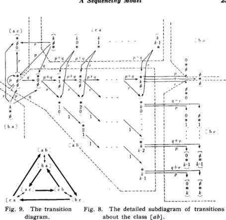
Then the transition diagram of the Markov chain can be written as Figures 8 and 9. Fig. 8 shows a part of it about the class [abJ, and Fig. 9 shows the relations between classes. A transition from a state in [ijJ to a state in

[jIJ

(i, j, l=a, b, e; i* j, j*l) implies a tran-sition of

*

from Si to Sj, or a change of the type of service from type

i to type j. Hence in order to obtain the limiting ratios of switches of the type of service, we may try to obtain the rate of transitions

Fig. 9. The transition diagram.

from one class to another. Numerical Examples. ~ c a , I I

" Z

", ~

~*===:'t:'

:;"*t.

u -

~ ~-

-p+" *1=

q---*--->- '; : /:/

~ ~

, "-.. I ( '

*

: I 0

;

=~:=~: =='1::;-c='=~ ::;-~ o : : I I I I I I I I I I I I I I I I o * 1 * 1

*

I I q+r

~ kk2==~!r=t!==~p~~~---.:

1~ I 1

*

*

I I k-l k-l I : q+r : : : p

+

k

1 : I I I

,'- ________ J

!

I I o

*

k

7

*

k ~ b c L ______________ _

Fig. 8. The detailed subdiagram of transitions about the class (ab).

The limiting ratios of switches of the type of service are calculated by using a computer. At that time, the idea of a lumped Markov chain was used to shorten the computing times (on this subject, see [2]). As a measure of the utility of the sequencing, we use the ratio

r

of the mean service time under Policy If to that under the first-come first-served policy (FCFS).

r

is also the reciprocal of the ratio of the capacity under Policy If to that under the first-come first-served policy.

r S _{Sunder FCFS} under Policy r

S.=Sb=S,=T,,=2

Tab= Tbc=l n.=T,,=T,b=O

p

Fig. 10. The ratio r of the mean service time under Policy I' to that under the first-come first-served policy for k=4.

(I' r) r---:-;----..,----,--- ( 0 0 ) - - - (.29.70.01) (.30.50.20) (.33.33.33) (.50.20.30) (.50 0 .50)

Fig. 11. The change of the ratio r for small k.

when k=4, Sa=Sb=Sc= T ac=2, T ab= Tbc=l and Tba= T ca = TCb=O, where

Si (i=a, b, c) is the net service time required by a customer of type i,

shows that in the case the sequencing gives an increase in the capacity of about 10 per cent. Fig. 11 shows the change of the value of the ratio

r

for small k. The curve with (.5, .0, .5) is the lower bound of

r.

The upper bound is the line

r=

1. 8. Remarks

Here some remarks on generalizations of the model are noted. Remark 1 is concerning the fundamental assumptions, and Remark 2 is concerning the restrictions of policies. Some remarks on a Markov chain method for a system with four or more types of customers are stated in Remark 3. In Remark 4, some remarks are noted for the case that the runway is used for both landings and takeoffs.

Remark 1.

We can treat a model with looser assumptions than those stated in the first paragraph of Section 3. In order to discuss about opti-mality of policies, net service times required by customers need not have the same lengths. We can argue in a similar way for the optimality of policies with no restriction on the net service times. Transfer times from one type to another may be possibly dependent (but independent with net service times) random variables with a common expectation if we loose the definition of the optimality so that it is preferable to minimize the expectation E(5) of the mean service time.

In order to calculate the limiting mean service time, we need some conditions for the renewal theorem. For example, we may re-quire that the net service times of type 0, the net service times of type 1, the transfer times from type 1 to type 0 and the transfer times from type 0 to type 1 are mutually independent random vari-ables having common distributions with finite expectations respectively.

The assumption that all the customers under consideration have already arrived and are waiting in a queue at the outset, is necessary only for the assurance of the adoptability of any policy in Pi. If we

consider our model under the restrictions Rl or R2, it is sufficient to assume that at least k customers are waiting in the queue at any time, since Im,,-nl;;:;;k under any policy in H.

Remark 2.

Besides the restrictions Ro, Rl, R2 and R3, we can conceive of other ones such as

RI: m,,~n-k for all n.

This assumption RI would not be adequate for the speed class se-quencing in the air traffic control. However we would be able to use this assumption for a servicing system with a finite waiting room.

We can also generalize restrictions Ri (i=1, 2, 3, 4) so that k is different according to types of customers.

Ri: m,,<mn+iGoH for all n such that e,,=O and for all i (>0).

mn<m"+iG,+i for all n such that en=1 and for all i (>0).

R'· 2· Imn-nl;;:;;ko for all n such that e,,=O.

Imn-nl;;:;;b for all n such that en=1.

R'· 3· mn;;:;;n+ko for all n such that en=O.

mn;;:;;n+kl for all n such that e,,= 1.

R'·

..

mn~n-ko for all n such that en=O. mn~n-b for all n such that e,,=1.

The limiting ratio a of 1--0 switches under an optimal policy under the restriction R; can be obtained similarly. Their results are as follows.

Restriction a

pq/(l +(ko+ k,)pq) pq/(l

+

pqE(ZkOk,

+

Zk,k_o)) pq/((ko+ l)p+(k,

+

l)q)

where Zkk' is a random variable having the following distribution. If

and if k>k', k'-1 P q

I

(

t -1 ) t-k' k' P{Zkk,=t}= ( t-l ) k t-k (t--l) t-k' k' k-l pq

+

k'---1 P q

o

Remark 3. (k;;'J<k') (k' ;;'J~ k

+

k' -1) (otherwise), (k~t~k+k'-I) (otherwise) .

The example in Section 7 can be generalized for systems with four or more type of customers. The limiting ratios of switches between servicing types can be analyzed similarly using Markov chains. For a system with four types of customers, states of a Markov chain are represented in quadruples of states of individual types. These states of individual types and transition rules between them are the same as in Section 7_ Then the transition diagram for the Markov chain has twelve parts and becomes more complicated.

Remark 4.

This sequencing model gives an information concerning the change of the capacity of a runway under the speed class sequencing in the air traffic control. However this model assumes that the runway is used for landings only. If the runway is used for both landings and takeoffs, we can use this model to analyze the capacity of the runway under the sequencing between landings and takeoffs. However if we want to analyze the capacity under the speed class sequencing for landings, there arises another problem concerning the priorities of landing aircraft and we must set up a more complicated model.

Acknowledgement

The author wishes to thank Mr. Akio Kato for his suggestion of this problem and Professor Hidenori Morimura for his advice and encouragement.

References

[1] Blumstein. A .• "The landing capacity of a runway." OPerations Research. 7 (1959). 752-763.

[2] Takahashi. Y .• "A lumping method for numerical calculations of stationary distributions of Markov chains" (in preparation).