Panel Data Research Center, Keio University
PDRC Discussion Paper Series
相対所得と生活満足度:誰が自分の所得を誰の所得とどの程度比較するのか?
白石 憲一、隅田 和人、上村 一樹、岡本 翔平、駒村 康平
2019 年 10 月 14 日
DP2019-002
https://www.pdrc.keio.ac.jp/publications/dp/5498/
Panel Data Research Center, Keio University
2-15-45 Mita, Minato-ku, Tokyo 108-8345, Japan
[email protected]
14 October, 2019
相対所得と生活満足度:誰が自分の所得を誰の所得とどの程度比較するのか? 白石 憲一、隅田 和人、上村 一樹、岡本 翔平、駒村 康平
PDRC Keio DP2019-002 2019 年 10 月 14 日
JEL Classification: I31
キーワード: 生活満足度;固定効果順序ロジット;距離の逆数;相対所得;準拠集団 【要旨】 第二次世界大戦終了後、一人当たり所得が増加しているにもかかわらず、西洋諸国と日本の平 均的な幸福度や生活満足度は上がらないという逆説に対して、相対所得はこの逆説を説明する 鍵と考えられている。この研究では、比較所得を相対所得の尺度として使用し、ミクロ計量経 済分析を行うことで、生活満足度の観点から比較所得の係数の符号を検証している。この研究 の貢献として、以下の 3 点を挙げることができる。第 1 は、固定効果順序ロジットモデルを用 いて、生活満足度の方程式を推定することである。第 2 に、準拠集団の平均所得を推計するた めに、居住する地域間の距離の逆数を重みとして使用している点である。第 3 に、所得比較の 方向と強さを同時に分析する点である。2011 年から 2017 年までの 20 歳以上の日本人のサンプ ルを分析する。等価世帯所得を説明変数として使用した分析結果から、サンプル全体と低所得 グル-プの比較所得の係数の符号は、ほぼすべてのケースで負である。したがって、効用の基 数性を仮定せずに個人レベルの固定効果をコントロ-ルし、さらにいくつかの個人および地域 の属性に基づいて準拠集団を定義しても、他人がより多くの収入を得ると、人々は相対的な剥 奪の感情を持つことを実証的に明らかにした。 白石 憲一 群馬医療福祉大学社会福祉学部 〒371-0823 群馬県前橋市川曲町191-1 [email protected] 隅田 和人 東洋大学経済学部 〒112-8606 東京都文京区白山5-28-20 [email protected]
上村 一樹 甲南大学マネジメント創造学部 〒663-8204 兵庫県西宮市高松町8-33 [email protected] 岡本 翔平 慶応義塾大学大学院 〒108-8345 東京都港区三田2-15-45 [email protected] 駒村 康平 慶応義塾大学経済学部 〒108-8345 東京都港区三田2-15-45 [email protected] 謝辞:久米功一博士と野崎華世博士に有益なコメントをいただいた。慶應義塾大学は 日本
家計パネル調査 Japan Household Panel Survey (JHPS/KHPS) の二次デ-タを提供していただ いた。心より感謝申し上げます。
Relative income and life satisfaction: Who compares their
income to whose income and to what extent?
Kenichi Shiraishi1, Kazuto Sumita2, Kazuki Kamimura3, Shohei Okamoto4 and Kohei Komamura5 1 Department of Social Welfare, Gunma University of Health and Welfare; 191-1, Kawamagari-machi, Maebashi-shi, Gunma, 371-0823, Japan
2 Department of Economics, Toyo University; 5-28-20, Hakusan, Bunkyo-ku, Tokyo, 112-8606, Japan 3 Hirao School of Management, Konan University; 8-33, Takamatsu-cho Nishinomiya, Hyogo, 663-8204, Japan
4 Graduate School of Economics, Keio University; 2-15-45, Mita, Minato-ku, Tokyo, 108-8345, Japan 5 Department of Economics, Keio University; 2-15-45, Mita, Minato-ku, Tokyo, 108-8345, Japan ORCID: Kenichi Shiraishi (0000-0001-6656-9564), Kazuto Sumita (0000-0001-7791-356X), Kazuki Kamimura 0002-4404-799X), Shohei Okamoto 0002-8580-5291), Kohei Komamura (0000-0001-9955-5943)
Corresponding author: Kenichi Shiraishi (e-mail: [email protected], TEL: +81-27-253-0294)
Acknowledgment: We thank Dr. Kouichi Kume and Dr. Kayo Nozaki for their helpful comments. Keio University provided the secondary data on 'the Japan Household Panel Survey and the Keio Household Panel Survey.'
Abstract: Relative income is considered a key to explain the paradox that, since the end of the Second World War, an increase in per capita income does not raise the average happiness or life satisfaction in western countries and Japan. This study uses comparison income as the measure of the relative income and verifies the sign of the coefficient of comparison income in terms of life satisfaction by conducting micro-econometric analysis. This study offers three main contributions. The first is to estimate the life satisfaction equation by using the fixed effects ordered logit model, which previous studies rarely consider. Second, to estimate the average income of the reference group, we use the inverse of the distance between the residential areas as the weight, which is new to the literature. Third, we analyze the direction and intensity of the income comparison simultaneously. We analyze a Japanese sample aged 20 or over in seven waves from 2011 to 2017. The results yield several findings. The sign of the coefficient of comparison income for the overall sample and low-income group is negative in almost all cases, using equivalent household income as an explanatory variable. Therefore, people may have feelings of relative deprivation when others earn more income, even if we control for individual fixed effects without assuming the cardinality of utility and define the reference group using several individual and regional attributes.
Keywords: Life satisfaction, Fixed effects ordered logit model, Inverse of distance, Relative income, Reference group
1. Introduction
Since the end of the Second World War, an increase in per capita income does not increase average happiness or life satisfaction in western countries and Japan. This phenomenon is also known as the Easterlin paradox (Easterlin 1974; Easterlin 1995). While this contradicts the assumption in traditional economics that the marginal utility of income is positive, the concept of relative income can explain these phenomena. Relative income, which denotes the income level as compared with one’s past income or that of others, affects happiness through adaptation or social comparisons. The effect of income increase on happiness is temporary and gradually disappears through adaptation. Social comparisons are related to both the perception of self and others. In this study, we focus on the relationship between social comparison and life satisfaction. Many studies highlight the importance of relative income as a determinant of the level of happiness when one’s income is compared to that of other important people. Even if an individual’s income rises, the individual’s level of happiness might decrease when people in the surrounding areas get an income raise comparatively equal to or more than that of the individual.
In economics, policy implications change depending on whether variables of relative income are specified in the utility function.1For example, if an increase in one’s consumption decreases the happiness of others and, therefore, has negative externality, the degree of distortion of the progressive income tax and the consumption taxation varies depending on whether relative income is considered, and structures of optimal taxation
1 Clark, Frijters, and Shields (2008) presented the implications for economic theory and policy design which consider relative income of social comparisons and adaptation issues in relation to economic growth, labor supply, wage profiles, optimal taxation and consumption, savings and investment, and migration.
may be altered. Furthermore, the poverty line is to be set differently depending on whether relative income is considered. Thus, it is imperative to understand how relative income affects individuals’ happiness empirically.
Empirical formulations of relative income in the subjective well-being equation can be classified into two methods. One method uses the income of the reference group as a comparison income (McBride 2001; Luttmer 2005), while the other uses the income evaluated relative to the reference group as a relative income (Ferrer-i-Carbonell 2005; Oshio, Nozaki, and Kobayashi 2011).2 Rather than relative income, comparison income as an explanatory variable is desirable to avoid multicollinearity between relative income and own income.
However, there is still no consensus on the sign of the coefficient of comparison income. We can explain this lack of consensus as due to the difference in probable mechanisms. Senik (2004) points out the existence of both the negative effect of comparison effects and the positive effect of information effects. Comparison effects are related to jealousy. Information effects are related to an ambition or signal effect, and the income of the reference group contains its future prospects. She points out that the role of information depends on the degree of the rapidly changing context where the relative position is unstable. Kingdon and Knight (2007) point out the possibility of positive and negative effects concerning the sign of the coefficient of comparison income. Feelings of relative deprivation such as envy, aspirations, and shame constitute a negative effect. However, a positive effect involves (1) altruism or fellow consciousness, (2) share of risk
2 The examples of relative income include the difference between own income and the comparison
within the community, and (3) proxy variables of social wage (such as the enhancement of local public goods). They highlight that people are altruistic towards others in a close community. Studies such as those by Senik (2004), Senik (2008), and Kingdon and Knight (2007) find positive effects from comparison income. However, many empirical studies find negative effects of comparison income (Blanchflower and Oswald 2004; Clark and Oswald 1996; Ferrer-i-Carbonell 2005; Luttmer 2005).
Furthermore, there are various unresolved issues regarding the methods in previous studies, which includes the estimation methods, the definition of the reference group, and the direction and intensity of income comparison. First, personality is mentioned as a major determinant of subjective well-being (Frey and Stutzer 2002). If there is a correlation between the unobserved personal attributes and explanatory variable, this correlation will result in a coefficient bias. Thus, to control such unobserved heterogeneity, we should use an estimation method that controls individual fixed effects, though many empirical examples do not do so (Blanchflower and Oswald 2004; Clark and Oswald 1996; Kingdon and Knight 2007; McBride 2001; Oshio, Nozaki, and Kobayashi 2011; Oshio and Urakawa 2012; Mizuochi 2017). Some studies estimate a linear fixed effects model by implicitly assuming the cardinality of utility (Clark, Westergard-Nielsen, and Kristensen 2009; Luttmer 2005; Senik 2008).3 Prior empirical studies that do not assume cardinality try to avoid the correlation between the individual random effects and the explanatory variables by using subjective well-being data of an ordinal scale having three or more
3Ferrer-i-Carbonell and Frijters (2004) report that if the fixed effects are controlled in the happiness function,
the results do not change substantially between linear and nonlinear estimation. However, it is not verified with various data sets in various countries.
values.4 Ferrer-i-Carbonell (2005), Senik (2004) and Urakawa and Matsuura (2007) estimate the ordered probit model which incorporate the Mundlak transformation by assuming that individual random effects depend on the mean values of explanatory variables proposed by Mundlak (1978). In practice, however, the relationship between individual random effects and the time-varying explanatory variables is not necessarily linear. In such a case, Mundlak type estimators may yield inconsistent and inefficient estimators in nonlinear models like logit, probit, and ordered probit and logit (Goetgeluk and Vansteelandt 2008; Brumback, Dailey, Brumback, Livingston, and He 2010).
Second, regarding the definition of the reference group, some studies define reference groups in terms of attributes such as individual attributes (McBride 2001; Oshio, Nozaki, and Kobayashi 2011), regional attributes (Blanchflower and Oswald 2004; Luttmer 2005; Clark, Westergard-Nielsen, and Kristensen 2009), and occupational attributes (Clark and Oswald 1996; Senik 2004; Senik 2008). A few prior studies define reference groups in terms of both the residential regional attributes and individual attributes. However, we define groups by both regional attributes and individual attributes in detail. Prior studies did not do so to avoid small sample sizes for the reference group (Ferrer-i-Carbonell 2005; Kingdon and Knight 2007). For example, Ferrer-i-Carbonell (2005) divide their sample by education and age group into five categories, but divide the regions into only West and East Germany.
Third, few studies analyze the direction and intensity of income comparison regarding subjective well-being simultaneously except Clark and Senik (2010), where
4Brown, Gray, and Roberts (2015) estimate the effect of comparison income with fixed effects ordered logit
several limitations exist. Clark and Senik (2010) fail to obtain the income of the reference groups and compare the income of the individual with that of the reference group. For example, their analysis shows that people who compare themselves with colleagues have significantly higher happiness levels than those who compare themselves with friends and the general public. However, there is a possibility that the average income of colleagues is lower than that of other reference groups. We cannot verify this conjecture as there is no direct information on the income of different reference groups. Furthermore, since the estimation method is based on the ordinary least squares estimation using the cross-section data, the fixed effects are not controlled.
This study empirically verifies the sign of the coefficient of comparison income and clarifies the parties involved in the comparison of one’s income with that of others and the extent to which the comparison is made. We estimate the life satisfaction equation using Japanese panel data and carefully verify the validity of the method of identifying elements such as variables, the scope of the reference groups, and the method of estimation. In this research, we conduct a micro-econometric analysis of life satisfaction and mainly analyze the effect of comparison income on it. The main contributions of this study in relation to previous works are as follows. First, this study performs an estimation with the fixed effects ordered logit model, which few studies employ. Therefore, it is unnecessary to assume the cardinality of utility, and it is possible to control unobserved time-invariant heterogeneity such as personality, which is regarded as a major determinant of life satisfaction. Controlling unobserved heterogeneity is very important to avoid bias in the coefficient estimates or spurious correlation. Moreover, we deal with the potential endogeneity of the reference group in part to verify the effects of comparison income on
life satisfaction. In other words, we perform an additional analysis that limits observations to non-movers to deal with the endogenous nature of the reference group.
Second, this study defines the reference groups by considering both detailed residential area and individual attributes. As a regional attribute, the average neighboring income is calculated based on the inverse of the distance between the residential areas of the respondents as a weight.5It is possible to calculate the neighboring income naturally on a nationwide basis by attaching a heavier weight to the observation in the near area. Moreover, by calculating the average of the neighboring income weighted by the inverse of the distance by conditioning the individual attributes, we can also define the reference groups reflecting not only the residential area in details but also the individual attributes such as gender, age, and educational background.
Third, this study analyzes the direction and intensity of income comparison simultaneously. Therefore, we divide the research work into three main parts to clarify who
compares their income to whose income and to what extent. First, regarding who, we
estimate the life satisfaction equation based on the samples divided by individual attributes. Next, regarding whose income, the average income is calculated by defining the reference groups according to 11 attributes on spatially weighted individual attributes, individual attributes, regional attributes, spatially weighted occupational attributes, and spousal attributes. Regarding to what extent, we compare the estimates of the coefficients of comparison income based on a linear fixed effects model, which is easy to compare.
The structure of this study is as follows. Section 2 explains the analysis method and the characteristics of this research by making comparisons with the previous studies. Section 3 explains the data employed. Section 4 estimates the life satisfaction equation with the whole sample, as well as the divided samples, and empirically clarifies who
compares their income to whose income and to what extent. Section 5 concludes.
2. Methods
In this research, we conduct a micro-econometric analysis of life satisfaction and mainly analyze the effect of the comparison income on it. There are two primary methods to calculate the comparison income. The first method is to estimate the wage equation and calculate the income estimate for each individual, which is the method used by researchers like Clark and Oswald (1996). The second method is to define the reference group and calculate the average or median value, which is the method used in studies like Ferrer-i-Carbonell (2005). This latter method is further divided into two methods; one that calculates the estimate from internal data and the other from external data. We use the average income of the reference group in calculating the comparison income from the internal data. In the following section, we describe the analysis methods.
2.1 Empirical model
We estimate a model with the following latent variable as the dependent variable. 𝑦𝑖𝑡∗ = 𝛼1𝑎𝑖𝑖𝑡 + 𝛼2𝑐𝑖𝑖𝑡+ 𝑥𝑐𝑖𝑡′𝛽 + 𝑐𝑖+ 𝜀𝑖𝑡, 𝑖 = 1, … , 𝑁, 𝑡 = 1, … , 𝑇. (1) Here, 𝑦𝑖𝑡∗ is a latent variable indicating the life satisfaction of individual i at time t. The observable variable is a discrete variable of the ordered scale, taking a value from 1 to 10 as follows:
𝑦𝑖𝑡 = 𝑗(j = 1, ⋯ , 10) if mj−1 < 𝑦𝑖𝑡∗ ≤ 𝑚𝑗 , where m0 = −∞ and m10= ∞.6 𝑎𝑖
𝑖𝑡 is a variable for own income, and 𝑐𝑖𝑖𝑡 is a variable
for the comparison income. Furthermore, 𝑥𝑐𝑖𝑡 is a vector of control variables, 𝑐𝑖 denotes
the unobserved individual heterogeneity that affects life satisfaction, and 𝜖𝑖𝑡 is a stochastic
error term. We are interested in the coefficient of comparison income, 𝛼2. We expect that this coefficient will be negative if the comparison effects are dominant and positive if the effects related to attributes such as altruism, regional public goods, and information effects are dominant. In the case of the reference group based on spatially weighted individual attributes, regional attributes, and spatially weighted occupational attributes, the comparison income is a weighted average of the income of the respondents living in the vicinity within a d km radius from the respondents. It is calculated as follows:
𝑐𝑖 = 𝑤𝑔(𝑑)× 𝑎𝑖,
where 𝑤𝑔(𝑑) is the spatial weight matrix and the (j, k) element of the matrix is the inverse
of the distance between the central point7 of municipality j, where the respondent i lives and that of municipality k where the respondent who belongs to the reference group g lives. The row elements are normalized such that they sum to 1 by convention. The element of this spatial matrix is 0 if the distance is over d km or survey year is different. Moreover, 𝑐𝑖 and 𝑎𝑖 are vectors of the comparison income and own income. In the case of the reference group based on regional attributes, d is defined as 30 km. In the case of the reference group based on spatially weighted individual attributes and spatially weighted occupational
6 Though life satisfaction from the questionnaire can be from 0 to 10, it is not possible to make stable estimations as the proportion of the observations with life satisfaction levels of 0 and 1 is small. Thus, these values are integrated into one value.
attributes, d is defined as infinity. Since a heavier weight is attached to the observation in the near area, we believe the reference groups based on spatially weighted individual attributes and spatially weighted occupational attributes also reflect regional attributes. We will describe the reference groups of respondents in detail later. The estimated parameters will be biased if the unobserved personal attributes affect life satisfaction and the explanatory variables; thus, we adopt the fixed effects ordered logit model to control unobserved time-invariant heterogeneities such as personality factors.
2.1.1 Estimation method of fixed effects ordered logit model by the MDE
model
The fixed effects ordered logit model is estimated using the method of Das and van Soest (1999) (hereinafter referred to as the Minimum distance estimation or MDE model) and the method proposed by Mukherjee, Ahn, Liu, Rathouz, and Sanchez (2008) (hereinafter referred to as the Blow-Up and Cluster or BUC model). In the MDE model, we perform the following two-step estimation. In the first step, by combining the adjacent categories of yit, taking values from 1 to 10, it is possible to compute nine pairs of the
binary variables, 𝑆𝑗,𝑖𝑡 (j = 2, 3 , ... 10), and estimate the fixed effects logit model of Chamberlain (1980) for each.
𝑆𝑗,𝑖𝑡∗ = 𝑥𝑖𝑡′𝜃𝑗+ 𝑐𝑖 + 𝜀𝑗,𝑖𝑡, 𝑖 = 1, … , 𝑁, 𝑡 = 1, … , 𝑇, (2)
where 𝑥𝑖𝑡 is a vector of explanatory variables including own income and comparison
income. In this model, we assume that 𝜖𝑗,𝑖𝑡 independently follows the logistic distribution and estimate the following conditional logit model.
𝑃𝑖𝑗(𝑆𝑗,𝑖1, … , 𝑆𝑗,𝑖𝑇|𝑥𝑖1, … , 𝑥𝑖𝑇, 𝑐𝑖, 𝑠𝑗,𝑖) = ∏𝑇 exp(𝑆𝑗,𝑖𝑡𝑥𝑖𝑡′ 𝜃𝑗) 𝑡=1 ∑ ∏ exp(𝑑𝑗,𝑖𝑡𝑥𝑖𝑡′𝜃 𝑗) 𝑇 𝑡=1 𝑑∈𝐷𝑗,𝑖 . (3)
Here, 𝑠𝑗,𝑖 indicates the sum of 𝑆𝑗,𝑖𝑡 that the i-th individual can take in the T periods, and we analyze 𝑆𝑗,𝑖 = (𝑆𝑗,𝑖1, … , 𝑆𝑗,𝑖𝑇) on the condition that the sum of T binary outcomes is 𝑠𝑗,𝑖. Furthermore, defining the set 𝐷𝑗,𝑖 = {𝑑𝑗,𝑖 |𝑠𝑗,𝑖 = ∑𝑇𝑡=1𝑑𝑗,𝑖𝑡} to have all possible combinations of 𝑠𝑗,𝑖 with a value of one and 𝑇 − 𝑠𝑗,𝑖 with a value of zero, we obtain a conditional likelihood function. However, due to this formulation, individuals who do not take 0 or 1 at all during the observation period are excluded from data analysis. We estimate this model for nine pairs of binary variables and find nine pairs of 𝜃̂𝑗. In the second stage, we can obtain β and its variance-covariance matrix using the minimum distance estimator for the common elements of the estimated parameters as follows. The estimates obtained in the first step are stacked in the column direction, and 𝜃̂ = (𝜃̂2′, 𝜃̂
3′, ⋯ , 𝜃̂10′ )′ is obtained. This result is a 9 ∙ K × 1 column vector, where K is the
number of regressors. Given the common element 𝛽 in 𝜃̂𝑗, in MDE, we will estimate 𝛽 by
minimizing
D(𝛽) = (𝜃̂ − 𝐻𝛽)′𝑉[𝜃̂]−1(𝜃̂ − 𝐻𝛽).
Here, H is a matrix of nine stacked K-dimensional identity matrices, and V[𝜃̂] is the variance-covariance matrix of the stacked estimation in the first stage. We can obtain the MDE of 𝛽 and its variance-covariance matrix as follows:
𝛽̂ = (𝐻′𝑉[𝜃̂]−1𝐻)−1𝐻′𝑉[𝜃̂]−1𝜃̂,
Here, we use 𝛽̂ as an estimate of the fixed effects ordered logit model by the MDE model.
2.1.2 Estimation method by the BUC model
The BUC model is a method proposed by Mukherjee, Ahn, Liu, Rathouz, and Sanchez (2008). As with the estimation method of the MDE model, by grouping the adjacent categories, nine pairs of estimates maximize the likelihood function imposed by the constraints in which the estimated values of the respective coefficients to explain the variables 𝑆𝑗,𝑖𝑡 (j = 2, 3, ... 10) are the same.
LBUC(𝜃) = ∑ ∑ 𝑙𝑛{𝑃𝑖𝑗(𝑆𝑗,𝑖1, … , 𝑆𝑗,𝑖𝑇|𝑥𝑖1, … , 𝑥𝑖𝑇, 𝑐𝑖, 𝑠𝑗,𝑖)} 𝑁 𝑖=1 10 𝑗=2 . (4)
Here, 𝑃𝑖𝑗 is the conditional logit model (3). In this estimation, the restriction that 𝜃̂2 = ⋯ = 𝜃̂10= 𝛽̂ is imposed, where 𝛽̂ is the estimator of the fixed effects ordered logit model by
the BUC model.
2.2 Defining the reference groups
We define the reference groups using spatially weighted individual attributes, individual attributes, regional attributes, spatially weighted occupational attributes, and spousal attributes. The average income of the reference group is calculated individually, assuming that the members of the reference group with whom comparison is made vary for each. Previous studies often performed analysis, assuming that the average income of the reference group is the same within the members of the same reference group. However, in reality, such a group should be different for individuals, being more affected by neighbors than those living at a distance. For example, even in the same prefecture, the residents in
cities or towns near Tokyo are affected by the residents in Tokyo’s metropolitan area while the residents in suburban cities or towns are likely affected by the residents in local prefectures. Therefore, we calculate the average income of the neighbors by using the inverse of the distance from the municipality where other households reside and use it as the comparison income.
2.3 Explanatory variables
Next, we elaborate on the explanatory variables of life satisfaction. Frey and Stutzer (2002) suggest the following five factors are determinants of happiness: 1) Personality factors, 2) Socio-demographic factors, 3) Economic factors, 4) Contextual and situational factors, and 5) Institutional factors.
Personality factors are particularly influenced by two factors, which are
temperament predisposition and traits and cognitive dispositions. In this study, since we
conduct the analysis by controlling the individual fixed effect, we can control personality when it does not change during the follow-up.
Age, gender, marital status, and educational background constitute the socio-demographic factors. Several studies report that happiness has a U-shaped relationship with age, and we included the squared terms of age, as well as age in logarithmic form. We also included marital status in our model.
Economic factors include income, unemployment, and inflation rate. We assume that not only own income, but also comparison income, affect happiness. We define comparison income as the income of a closely related group. We use unemployment as a
dummy variable because unemployment affects life satisfaction significantly, even though other variables are controlled.
Contextual and situational factors refer to human relations, health, and employment conditions. We add the average volunteer participation rate of the neighbors as proxy variables of social capital and add health and work status as explanatory variables.
Institutional factors include the political system and governance to the government. In this study, we control the effects of the institutional factors indirectly by including year dummies as explanatory variables since it reflects changes in the institutional factors.
3. Data
3.1 Japan household panel survey
We use the Japan Household Panel Survey (JHPS/KHPS) to estimate the model. This survey is a combination of the former Japan Household Panel Survey (JHPS) and the
Keio Household Panel Survey (KHPS), which were previously conducted and managed as
separate surveys. The characteristics of the surveys, such as the data structure and sample, are as follows.8
The KHPS began in 2004, surveying 4,005 households, and the JHPS began in 2009 surveying 4,000 households. Approximately 1,400 and 1,000 new panel members of the KHPS are recruited in 2007 and 2012 respectively. In both surveys, households are selected through a stratified two-stage sampling method throughout Japan. The survey
8 For precise information, see Panel Data Research Center at Keio University
subjects of the KHPS are selected from men and women aged 20 to 69 nationwide, and those of the JHPS are selected from men and women aged 20 or above nationwide. Although the sampling populations overlap, ultimately, there is no overlap of KHPS and JHPS respondents. The two data sets have been combined since 2015 as the JHPS/KHPS since they contain questions that are either the same or similar.
Poverty rate after taxes and transfers in Japan in 2015 is 15.7% according to the Organization for Economic Co-operation and Development (OECD) Income Distribution database, which is very high among the OECD countries. The poverty rate is calculated as the ratio of the number of people whose equivalent disposable income falls below the poverty line, which is half of the median equivalent disposable income of the total population. We will examine whether the effect of comparison income work on life satisfaction in countries with high poverty rates. We use seven waves of JHPS/KHPS run annually from 2011 to 2017; they contain a questionnaire about life satisfaction since 2011. Explanatory variables are created from the data of JHPS/KHPS. In the following sections, we describe how to prepare the variables of life satisfaction, income, social capital, and health condition. Table A1 and A2 in the appendix summarize descriptive statistics of variables used for the analysis.
3.2 Life satisfaction
In JHPS/KHPS, respondents are asked to rate satisfaction with their general life in 11 levels on a scale of 0 to 10: 0, not at all satisfied; 5, neither satisfied nor dissatisfied; and 10, fully satisfied. General life satisfaction is a validated scale to measure subjective
well-being, considering various aspects of satisfaction with life (such as finance, job, and health) (Praag, Frijters, and Ferrer-i-Carbonell 2003).
3.3 Income
Equivalent household income is calculated by dividing the total annual after-tax household income by the square root of the number of household members. We use the respondents’ total annual before-tax income as individual income.9 We obtain real income by creating a price index that reflects regional and intertemporal differences from the consumer price regional difference index (by prefecture) and the general index that excludes the imputed rent of owned house from the time series consumer price index (Japan, 2015=100). To calculate the average income of neighbors, we measure the distances between respondents and calculate the weighted average of the income of people from surrounding areas with the weights of the inverse of the distance. We use income surveyed in JHPS/KHPS in calculating the income of people from surrounding areas. Since JHPS/KHPS surveys the information about the city where individuals reside, using the
CSV address matching service provided by the University of Tokyo Spatial Information
Science Research Center, we obtained the latitude and longitude of the location of the city hall of the individual's place of residence, then we measured the distances between respondents.10
9 In JHPS/KHPS, respondent’s total annual after-tax income is not surveyed.
10According to Miura (2015), the distance between the residential areas is conveniently measured in the
following manner with the latitude as φ, the longitude as λ, and the number of the subscript as the point. L= 6370 arccos(sin φ1 sin φ2+ cos φ1 cos φ2 cos(λ1 − λ2))
We used gender, age range, full-time employment dummy, and a dummy for university graduates as attributes of individuals to be conditioned and to calculate the average income in the case of the reference groups of spatially weighted individual attributes, as well as individual attributes. The age range of the reference group is defined as five years younger and older than the individual concerned, as McBride (2001) proposes. For example, if an individual is 45 years old, the age range of the reference group is 40 to 50 years old.
We use the logarithmic value of the income of the reference group for comparison income. We expect a negative sign of the coefficient of comparison income if comparison effects occur and a positive sign if information effects or altruism occur. The explanatory variables for the analysis include: age and squared age of the respondent, own income, comparison income, participation rate of neighbors in volunteer work, spouse dummy, employment state (regular employee dummy, non-permanent employee dummy, self-employed person dummy, and unemployment dummy), homeowner dummy, health (psychosomatic symptom score), and year dummies. Time-invariant variables such as gender and educational background are not included in explanatory variables because the fixed effects are controlled.
The reference groups for income comparison in this study are based on spatially weighted individual attributes, individual attributes, regional attributes, spatially weighted occupational attributes, and spousal attributes.11 Furthermore, four types of spatially
weighted individual attributes, as well as individual attributes, are defined as the reference groups from the attributes of the respondents as follows:
(G1) (i) Age, (ii) Gender, and (iii) Marital status
(G2) (i) Age, (ii) Gender, (iii) Educational background, and (iv) Marital status
(G3) (i) Age, (ii) Gender, (iii) Occupational form, and (iv) Marital status
(G4) (i) Age, (ii) Gender, and (iii) Educational background
For the four types of spatially weighted individual attributes, we calculate the comparison income from the weighted average of the income of the neighbors with the same attributes for each of the four types using the inverse of the distance as the weight. For example, the reference group in (G1) consists of respondents who are in the age range of five years younger and older than the individual concerned and are of the same gender and have the same marital status using the inverse of the distance as the weight. Therefore, we measure the comparison income within the JHPS/KHPS data set without extrapolating from external data. Similarly, regarding reference groups (G2) to (G4), we calculate the average incomes of neighbors with the same attributes using the inverse of the distances as the weight.
We create a comparison income based on the regional attributes; that is, respondents within a 30 km radius for each respondent using the inverse of the distances as weight. The advantages and disadvantages of limiting the scope of the region as a reference group are as follows. The reference group can reflect regional attributes more strongly. However, the reference group will have fewer observations. The sample size becomes small because the reference group will have many conditions to consider in the
case of spatially weighted individual attributes and spatially weighted occupational attributes. Thus, the disadvantage of limiting the range of the area emerges strongly, and the spatial weight is created without specifying the range in those cases. Therefore, since the number of conditions to consider is small for reference groups based on regional attributes, we set 30 km as the distance to reflect strong regional attributes. Depending on the type of reference group, there is no uniformity in the scope of the region because we take the trade-off relation between the advantages and disadvantages into consideration.
Table 1 shows the number of respondents within a 30 km radius from the 10th percentile to the 99th percentile for all observations from 2011 to 2017. We calculate the result as follows:
𝑧 = 𝑤𝑖30× 𝐽,
where 𝑤𝑖30 is the spatial weight matrix. The (i, k) element of the matrix takes one if the respondent i lives within a 30 km radius from the municipality where respondent k lives in the same year; otherwise, it is 0.12 𝐽 is a vector where all elements are 1. By sorting the
number of the respondents living within a 30 km radius in ascending order, the number at the 10th percentile is 4, and 16 is at the 25th percentile point, in that order. The comparison income is treated as the missing value if no one lives in the above distance. Since the median of the respondents living within the 30 km radius is 53, the members of the reference group will be very small when we define a reference group by combining multiple attributes (individual, regional, and occupational attributes). For example, for (G1), a reference group based on spatially weighted individual attributes, we have to select
its members from the respondents within a 30 km radius with a median of 53 who are of similar age (age range of five years younger and older), the same gender, and the same marital status. That is, if we restrict the geographical scope within a 30 km radius. Thus, there may be no members in the reference group for some respondents. Therefore, we do not restrict the geographical scope for spatially weighted individual attributes and spatially weighted occupational attributes. However, we restrict the geographical scope within a 30 km radius in the reference group, which we define using only the regional attribute because many respondents have a certain number of members of the reference group. If the distance is much shorter than 30 km, the problem of small sample sizes of the reference group becomes severe, and if the distance is much longer than 30 km, the reflection of the regional attribute on the reference group may be weak. Thus, we define the area within a 30 km radius for the reference group of regional attributes.
Table 1: The number of respondents living within 30 km radius
The percentile point The percentile values of z
10% 4
25% 16
50% 53
75% 206
99% 835
Note: z is calculated as follows: 𝑧 = 𝑤𝑖30× 𝐽, where 𝑤𝑖30 is the spatial weight matrix. The element of the matrix takes one if the distance between the respondents is within 30 km and the survey year is same; Otherwise, it takes 0. 𝐽 is a vector where all elements are 1.
We create one type of comparison income based on spatially weighted occupational attributes by calculating the weighted average of the income of people from surrounding areas using the inverse of the distance as a weight. The following attributes define the
comparison subjects: (i) Age, (ii) Gender, (iii) Form of employment, (iv) Company size, and (iv) Nature of the work.
3.4 Social capital
Putnam (1995) defined social capital as “the characteristics of society such as network, norms, and trust that enhance social efficiency by encouraging people’s cooperative activities.” Previous studies report that social capital exerts a positive influence on an individual’s health and well-being (Matsushima and Matsunaga 2015; Murayama, Fujiwara, and Kawachi 2012). We can classify the methods to measure social capital into two dimensions: the individual level and the group level. As the individual level of social capital may be endogenous in relation to life satisfaction, we adopt the group-level social capital as an explanatory variable.
Specifically, we calculate the weighted average of the participation rate in volunteer activities amongst the people in the surrounding areas (1 if they participate almost every day or several times per week; 0, otherwise) with the weight of the inverse of the distance normalized such that it sums to 1. This calculation excludes individuals who reside at a distance of more than 30 km away from the respondent. Participation in volunteer activities is often used as a proxy variable of reciprocity, which is one component of social capital (Matsushima and Matsunaga 2015; Saxton and Benson 2005). In line with these existing findings, the greater the participation rate, the higher the altruism and reciprocity. We expect that social capital has a positive influence on life satisfaction.
3.5 Health condition
As a proxy variable for health, we can use the following three kinds of variables: (1) Self-rated health (SRH), (2) Objective health condition, and (3) Psychosomatic symptom score.
For SRH, the following question is asked in the survey: How is your health
normally? The respondent chooses one of the following: 1) Good, 2) Pretty good, 3)
Normal, 4) Not so good, and 5) Bad.
For an objective health condition, the following questions are asked: Did you
receive medical treatment, or were you hospitalized last year? and What types of problems
were noted in the examination results?
For the psychosomatic symptom score, questions pertaining to the symptoms are as follows: 1) Headache or dizziness, 2) Palpitations (or out of breath) 3) Digestive problems, 4) Back, lower back, and shoulder pain, 5) Tire easily, 6) Catch cold easily, 7) Often become irritated, 8) Trouble falling to sleep, 9) Find seeing people tiresome, 10) Lost work concentration, 11) Dissatisfied with life, and 12) Anxiety about the future. For each question, respondents select one of the following choices: 1) Never, 2) Rarely, 3) Sometimes, and 4) Often. The scores for these answers range from 0 for Never, 1 for
Rarely, 2 for Sometimes, and 3 for Often. The scores for the 12 answers are summed up
and are used as the psychosomatic symptom score.
Although SRH can be comprehensive enough to include overall health (Chandola and Jenkinson 2000), there is a risk of generating bias that would leave to a large coefficient. The risk arises because the explanatory variable of life satisfaction is also
subjective, and reverse causality and confounders (such as mood at that time) might be problematic. However, the objective health condition might capture only a portion of the health, and the bias due to measurement error may underestimate the coefficient of health.
Since the psychosomatic symptom score requires the symptoms, we expect that that mood and the environment at that time will have little effect. Thus, it may be more appropriate as the objective measurement of health than SRH and as the more comprehensive scale than the objective health condition variable. Thus, we use the psychosomatic symptom score as the variable for health conditions. However, caution is required as the scale focuses only on the limited negative aspects of the health condition, and it is not a complete proxy variable for the health condition.13
4. Results
In the following section, we estimate the life satisfaction equation with the whole sample, as well as the divided samples, by using the comparison income of the various reference groups mentioned above.
4.1 Analysis of the effect of comparison income
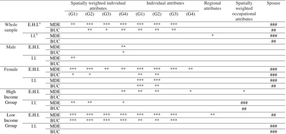
Table 2 summarizes the results of the estimated effects of the comparison income based on various reference groups which satisfy the significance level by using the whole sample and divided samples by gender and income group. Based on the seven-year average
13 Since we are not able to find appropriate instrumental variables, we do not perform an instrumental variables estimation in this study.
income, we classify the sample into a high-income group with above-average income and a low-income group with below-average income. The coefficients of the comparison income based on equivalent household income in the whole sample, females, and the low-income group tend to show comparison effects stably. However, the coefficients of the comparison income based on individual income show comparison effects in a few cases. We find comparison effects mainly in women when using equivalent household income as an explanatory variable because many women depend largely on their husband’s income in terms of living standards. The average total income of wives is about three-tenths of the average total income of husbands within married respondents of JHPS/KHPS.
By comparing coefficients of comparison incomes of various reference groups, the coefficients of the comparison income calculated from the equivalent household income of the individual attributes, (G1) and (G2), and the spatially weighted individual attributes (G4) show stable comparison effects; the direction of income comparison is different depending on whether or not to consider regional attributes as the reference group.
However, if we divide the sample by gender and income group, comparison effects are not observed for men except some reference groups. Moreover, comparison effects are observed in most cases for low-income groups using equivalent household income as an explanatory variable. However, comparison effects are not observed for the high-income group except for some reference groups. This observation implies that income comparison is not symmetric. That is, the increase of the average income of the reference group decreases the life satisfaction of the low-income group, but it does not affect the life satisfaction of the high-income group except for some reference groups. This result is consistent with the model advocated by Duesenberry (1949).
26
Table 2: The effects of comparison income, JHPS/KHPS 2011–2017
Spatially weighted individual attributes
Individual attributes Regional attributes Spatially weighted occupational attributes Spouse (G1) (G2) (G3) (G4) (G1) (G2) (G3) (G4) Whole sample E.H.I.a MDE ** *** *** *** *** *** *** ### BUC ** * ** ** ** ** ## I.I.b MDE * ### BUC ##
Male E.H.I. MDE **
BUC *
I.I. MDE **
BUC
Female E.H.I. MDE *** *** ** ** *** *** *** ** ###
BUC * * ** ** ### I.I. MDE *** *** ### BUC *** ** ## High Income Group E.H.I. MDE ** ** ** * * BUC I.I. MDE ** ** * ### BUC ## Low Income Group E.H.I. MDE *** *** *** *** *** *** *** ** ## BUC *** *** *** *** ** ** *** I.I. MDE ### BUC ###
Note: *Negatively significant at the 0.10 level; **at the 0.05 level; ***at the 0.01 level. #Positively significant at the 0.10 level; ##at the 0.05 level; ###at
the 0.01 level. There are four types of spatially weighted individual attributes and individual attributes as follows: (G1) (i) Age, (ii) Gender, and (iii) Marital status, (G2) (i) Age, (ii) Gender, (iii) Educational background, and (iv) Marital status, (G3) (i) Age, (ii) Gender, (iii) Occupational form, and (iv) Marital status, (G4) (i) Age, (ii) Gender, and (iii) Educational background.
a
E.H.I. means the case of equivalent household income.
b
For the reference group based on the regional attributes, we expect a negative coefficient if the comparison effects are dominant and a positive one if the effects of attributes such as altruism and regional public goods are dominant. Table 2 shows the negative effects in a few cases. Clark et al. (2009) and Mizuochi (2017) report a statistically significant positive effect, contrary to the findings of this study. Mizuochi (2017) restrict the sample to some areas in Japan, and thus, we might consider this sample as a special group. Further, since he does not control the fixed effects, the estimated coefficient may be biased. However, in this study, we set the area within a 30 km radius as the reference group. It is possible that the positive effects that relate to altruism occur only in narrow areas like residents’ associations or an elementary school districts where there are many opportunities for daily interaction, which is an important area for future study.
For the reference group based on the spatially weighted occupational attributes, we see positive effects in the high-income group when using individual income as an explanatory variable. We could interpret these positive effects as information effects. However, we observe no positive effects when using equivalent household income as an explanatory variable. One reason for this result for the high-income group is that the individual income of the reference group may contain their future prospects. However, the equivalent household income of the reference group may not contain their future prospects. For example, we imagine a hypothetical case of two husbands with similar occupational characteristics, as follows:
A: Yearly income the husband earns is 5,000,000 yen; the wife earns 200,000 yen.
The occupational attributes of the husband in the case of A are similar to those in the case of B. However, the occupational attributes of the wife in the case of A are not similar to those in the case of B. Thus, it seems natural to conclude that the household income in the case of B, which is more than twice as high as that in the case of A, does not contain future prospects for the husband in the case of A. This example can explain one reason why we do not see information effects when using equivalent household income as an explanatory variable. Even in a society like Japan, where relative position is stable, we find information effects for high-income group.
The analysis of spouses as the reference group shows positive effects opposite to the comparison effects in both the equivalent household income and the individual income. Although further investigation will be needed, we believe that it is reasonable to conclude that the income of a spouse that the respondent shares may affect life satisfaction positively.
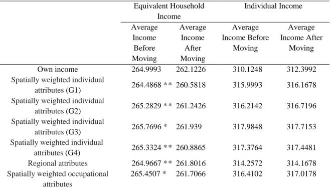
Next, the respondents who moved to a different city are removed to avoid the endogeneity of the reference group. The statistical significance for the coefficient of comparison income remains unchanged, and the difference in the estimation result is not large. Due to lack of space, we omit this analysis results, but these are available to readers on request. Table 3 presents the average income level of individuals and various reference groups before and after moving. In this table, we extract the observations of the same respondent for two consecutive years whose residential city is different. By averaging incomes in the former year of these observations, we can calculate the average income before moving. Moreover, by averaging incomes in the latter year of these observations, we can calculate the average income after moving. In the case of the equivalent household
income of the moving respondents, while the incomes of the household and the reference group both tend to decline somewhat after moving, the decline for the reference group is slightly sharper.
Table 3: Average income level of individuals and various reference groups before and
after moving, JHPS/KHPS 2011–2017 Equivalent Household Income Individual Income Average Income Before Moving Average Income After Moving Average Income Before Moving Average Income After Moving Own income 264.9993 262.1226 310.1248 312.3992
Spatially weighted individual
attributes (G1) 264.4868 * * 260.5818 315.9993 316.1678
Spatially weighted individual
attributes (G2) 265.2829 * * 261.2426 316.2142 316.7196
Spatially weighted individual
attributes (G3) 265.7696 * 261.939 317.9848 317.7153
Spatially weighted individual
attributes (G4) 265.3324 * * 260.8865 317.3764 317.4481
Regional attributes 264.9667 * * 261.8016 314.2572 314.1678
Spatially weighted occupational attributes
265.4507 * 261.7066 316.4102 317.0178
Note: The unit of currency is million yen. Asterisks indicate significant differences (Student's two-sided
t-test, ** p<0.01, * p<0.05). The column of Average Income Before Moving is the average income in the former year of the observations of the same respondent for two consecutive years whose residential city is different. The column of Average Income After Moving is the average income in the latter year of the observations of the same respondent for two consecutive years whose residential city is different. There are four types of spatially weighted individual attributes as follows: (G1) (i) Age, (ii) Gender, and (iii) Marital status, (G2) (i) Age, (ii) Gender, (iii) Educational background, and (iv) Marital status, (G3) (i) Age, (ii) Gender, (iii) Occupational form, and (iv) Marital status, (G4) (i) Age, (ii) Gender, and (iii) Educational background.
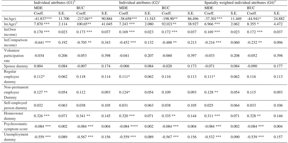
In Table 4, we discuss the result of analysis of equivalent household income and the reference groups with individual attributes, (G1) and (G2), and spatially weighted
individual attributes (G4). This result is the estimation results of the MDE model and the BUC model. This table shows comparison effects stably based on whole sample. The coefficient of comparison income is negative and statistically significant. The participation rate for volunteers, which is a proxy variable of social capital, is not significant. Life satisfaction is high for those earning high-income and living in self-owned housing and low for those unemployed, resulting in a high score for psychosomatic symptoms.
31
Table 4: Results in the case of equivalent household income and various reference groups in whole samplea, JHPS/KHPS 2011–2017
Individual attributes (G1)b Individual attributes (G2)c Spatially weighted individual attributes (G4)d
MDE BUC MDE BUC MDE BUC
Coeff. S.E. Coeff. S.E. Coeff. S.E. Coeff. S.E. Coeff. S.E. Coeff. S.E.
ln(Age) -41.837*** 11.700 -217.04** 90.884 -38.658*** 11.543 -198.90** 86.496 -37.301*** 11.469 -44.941* 24.882 ln(Age)2 7.870 *** 2.114 100.65** 41.045 7.243 *** 2.080 92.021** 38.927 6.966 *** 2.062 8.355 * 4.472 ln(Own income) 0.170 *** 0.023 0.173 *** 0.037 0.169 *** 0.023 0.172 *** 0.037 0.169 *** 0.023 0.172 *** 0.037 ln(Comparison income) -0.641 *** 0.192 -0.705 ** 0.343 -0.452 *** 0.132 -0.488 ** 0.213 -0.216 *** 0.060 -0.232 ** 0.096 Volunteer participation rate -0.034 0.206 -0.053 0.398 -0.041 0.207 -0.060 0.397 -0.033 0.208 -0.052 0.398 Spouse dummy 0.004 0.084 -0.007 0.174 -0.006 0.084 -0.020 0.173 -0.071 0.084 -0.090 0.177 Regular employee dummy 0.112* 0.062 0.118 0.114 0.111* 0.062 0.116 0.113 0.111* 0.062 0.116 0.113 Non-permanent employee Dummy 0.127 ** 0.054 0.112 0.093 0.124* 0.054 0.109 0.093 0.128 ** 0.054 0.115 0.093 Self-employed person dummy 0.032 0.063 0.038 0.105 0.031 0.063 0.038 0.105 0.025 0.064 0.033 0.106 Homeowner dummy 0.326 *** 0.071 0.341 ** 0.145 0.320 *** 0.071 0.335 ** 0.144 0.311 *** 0.071 0.328 ** 0.146 Psychosomatic symptom score -0.084 *** 0.002 -0.084 *** 0.004 -0.084 **** 0.002 -0.084 *** 0.004 -0.084 *** 0.002 -0.084 *** 0.004 Unemployment dummy -0.559 *** 0.089 -0.567 *** 0.156 -0.559 *** 0.089 -0.567 *** 0.156 -0.532 *** 0.090 -0.539 *** 0.157
Note: Significant level: *** p<0.01, ** p<0.05, * p<0.1. Time-dummies are present in all estimates but are not shown. a
The number of observations and the number of individuals varies depending on the cut-off point which dichotomizes the ordered variable of life satisfaction.
b
Individual attributes (G1) as the reference group are composed of respondents who are in the age range of five years younger and older than the individual concerned, are of the same gender, and have the same marital status.
32
c
Individual attributes (G2) as the reference group are composed of respondents who are in the age range of five years younger and older than the individual concerned, are of the same gender, and have the same educational background and marital status.
d
Spatially weighted individual attributes (G4) as the reference group are composed of respondents who are in the age range of five years younger and older than the individual concerned, are of the same gender, and have the same educational background using the inverse of the distance as weight.
4.2 Direction and intensity of comparison effects
We proceed to analyze the direction and intensity of the comparison effects. For the nonlinear estimation, we cannot simply compare the magnitude of the marginal effect from the estimated coefficients; thus, we compare the estimated coefficients of the comparison income in the linear fixed effects models. That is, we use the linear model to analyze who
compares their own income to others, who these others are, and to what extent. The
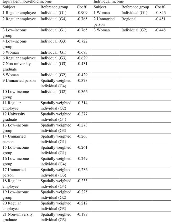
subjects are divided by gender, employment type (regular and irregular), educational background (university graduate and non-university graduate), marital status (married and unmarried) and income group (high and low). Table 5 summarizes the negative coefficient of the comparison income, which is statistically significant among the 11 reference groups mentioned above. For equivalent household income, the coefficients of comparison income are statistically significant at the five percent level in 21 cases. Moreover, regular employees and the low-income group tend to care about the average income of the reference groups defined by individual attributes. For individual income, the coefficients of comparison income are statistically significant at the five percent level in three cases, and women particularly care about the average income of the reference groups defined by individual attributes.
Table 5: Comparison of the effects of comparison income, JHPS/KHPS 2011–2017
Equivalent household income Individual income
Subject Reference group Coeff. Subject Reference group Coeff. 1 Regular employee Individual (G1) -0.909 1 Woman Individual (G1) -0.846 2 Regular employee Individual (G4) -0.765 2 Unmarried
person
Regional -0.451 3 Low-income
group
Individual (G1) -0.765 3 Woman Individual (G2) -0.448 4 Low-income
group
Individual (G3) -0.722 5 Woman Individual (G1) -0.673 6 Regular employee Individual (G3) -0.629 7 Non-university
graduate
Individual (G3) -0.431
8 Woman Individual (G2) -0.429
9 Unmarried person Spatially weighted individual (G4) -0.373 10 Low-income group Individual (G2) -0.366 11 Regular employee Spatially weighted individual (G2) -0.314 12 University graduate Spatially weighted individual (G4) -0.277 13 Low-income group Spatially weighted individual (G3) -0.273 14 Unmarried person Spatially weighted individual (G1) -0.263 15 Low-income group Spatially weighted individual (G1) -0.261 16 Low-income group Spatially weighted individual (G4) -0.249 17 Unmarried person Spatially weighted individual (G3) -0.236 18 Regular employee Spatially weighted individual (G4) -0.233 19 Low-income group Spatially weighted individual (G2) -0.225 20 Regular employee Spatially weighted individual (G3) -0.212 21 Non-university graduate Spatially weighted individual (G3) -0.188
Note: This is a summary of the negative coefficient of the comparison income, which is statistically
5. Conclusion
This study empirically verifies the sign of the coefficient of comparison income and investigate who compares their income to whose income and to what extent by conducting a micro-econometric analysis of life satisfaction. We control individual fixed effects without arbitrarily assuming the cardinality of utility by using the panel data from Japan, which reflect the population composition of society over the age of 20 considerably.
The results of our analysis are as follows. Concerning the sign of the coefficient of comparison income, whenever the coefficient is significant in whole sample, it is negative in almost all cases except when the spouse is the reference group. Therefore, comparison effects may be stronger. Meanwhile, in almost all cases, there are few positive effects, which are related to attributes such as information effects, altruism, and the enhancement of regional public goods. Comparison effects are observed in most cases for the low-income group, but they are not observed for the high-low-income group except some reference groups using equivalent household income as an explanatory variable. This observation implies that income comparison is not symmetric as with the model advocated by Duesenberry (1949). Therefore, people may have feelings of relative deprivation when others earn more income. However, there is no feeling of relative satisfaction when others earn less income in most cases, even if individual fixed effects are controlled for without assuming cardinality of utility and detailed individual and regional attributes are considered in defining reference groups. Only for the high-income group when using individual income as an explanatory variable do we see positive effects related to information effects.
This study has several limitations that provide opportunities for further research. First, it is necessary to measure the representative value of income by narrowing the area of the reference group and the range of occupational attributes. In that case, it would be necessary to select observations by random sampling from all over the country to eliminate local bias; the analysis with the panel data is desirable. For regional attributes as the reference group, it would be ideal to narrow the geographical scope to the level of daily interaction, such as residents’ associations and elementary school districts. For occupational attributes as the reference group, it would be ideal to match the data of individuals to their workplace and to measure the average income of colleagues of the same company.
Second, this study uses the weighted average of the participation rate of people in volunteer activities from surrounding areas as a proxy variable for social capital. For future research, it is necessary to explore the possibility of using more comprehensive indicators which reflect reliability and various elements contained in the social capital as used in Kim, Subramanian, Gortmaker, and Kawachi (2006).
In conclusion, comparison effects which relate feelings of relative deprivation, such as jealousy, envy, and shame, are observed to be significant for life satisfaction even if unobserved time-invariant heterogeneities and various reference groups are considered. Particularly, people may have feelings of relative deprivation when others earn more income because the low-income group tends to care about the average income of the reference group.
Compliance with Ethical Standards
Ethical approval was not required because this study was based on secondary analysis of publicly available data.
Conflict of Interest
Appendix
Table A1: Distribution of Life Satisfaction
Life satisfaction Frequency Percentage 0 (low) 486 1.68 1 376 1.3 2 786 2.71 3 2,059 7.11 4 2,401 8.29 5 7,955 27.47 6 3,244 11.2 7 4,341 14.99 8 4,564 15.76 9 1,753 6.05 10 (high) 997 3.44 Total 28,962 100
Table A2: Description statistics
Mean Standard deviation
Age 53.96772 14.66297
Spouse dummy 0.751122 0.43237
Non-permanent employee dummy 0.213315 0.409655
Self-employed person dummy 0.147898 0.355005
Homeowner dummy 0.816463 0.387113
Psychosomatic symptom score 11.31427 6.436945
Unemployment dummy 0.019123 0.13696
Volunteer participation rate 0.0776902 0.0471904
Equivalent household income 263.6326 210.1775
Individual income 310.4621 310.0594
References
Blanchflower, D. G., & Oswald, A. J. (2004). Well-being over time in Britain and the USA.
Journal of Public Economics, 88(7-8), 1359-1386.
Brown, S., Gray, D., & Roberts, J. (2015). The relative income hypothesis: A comparison of methods. Economics Letters, 130, 47-50.
Brumback, B. A., Dailey, A. B., Brumback, L. C., Livingston, M. D. & He, Z. (2010). Adjusting for confounding by cluster using generalized linear mixed models. Statistics
& Probability Letters, 80(21-22),1650-1654.
Chamberlain, G. (1980). Analysis of covariance with qualitative data. Review of Economic
Studies, 47(1), 225-238.
Chandola, T., & Jenkinson, C. (2000). Validating self-rated health in different ethnic groups. Ethnicity & Health, 5(2), 151-159.
Clark, A. E., Frijters, P., & Shields, M. A. (2008). Relative income, happiness, and utility: An explanation for the Easterlin paradox and other puzzles. Journal of Economic
Literature, 46(1), 95-144.
Clark, A. E., & Oswald, A. J. (1996). Satisfaction and comparison income. Journal of
Public Economics, 61(3), 359-381.
Clark, A. E., & Senik, C. (2010). Who compares to whom? The anatomy of income comparisons in Europe. The Economic Journal, 120(544), 573-594.