A Study on Natural Language Understanding Based on
Mental Image Directed Semantic Theory
by
BD14002
Rojanee Khummongkol
Engineering Doctor's Program
A dissertation submitted in partial fulfillment of
the requirements for the degree of
Doctor of Engineering
Intelligent Information System Engineering
Fukuoka Institute of Technology
Fukuoka, Japan
I
Acknowledgement
In order to accomplish my dissertation, first of all I would like to express my deep appreciation to Prof. Masao Yokota, Ph.D., my great supervisor for his guidance, enthusiastic encouragement and useful critiques of my research work during my study of doctor course in Japan and henceforth. He does not advise me only academic knowledge, but also remind me the way of life. However, I would not have succeeded in this attempt if I had lacked of opportunity from him to enter Fukuoka Institute of Technology (FIT) as a Ph.D. student with the support of education fund from my original affiliation, University of Phayao.
Moreover, I would like to extend my gratitude to Prof. Dr. Yu Song, Prof. Dr. Hiroyuki Fujioka, Prof. Dr. Hitoshi Kino, and others for their suggestion, advices and assistances. Also furthermore, I wish my grateful thanks to Mr. Hiroshi Chikamatsu, Ms. Sawako Tsunenoki, and Ms. Hiroko Yoshida, FIT staffs, who always help and embolden me to go over troubles. Besides, I am particularly sincere to thank my special guests, i.e. Janelle Chang, Christine C. Cabugao, Mingyue Qiu, Taiyo Nishiguchi, Jiraporn Pooksook, and my father (Chairoj Khummongkol) for their helps as a sample group in my psychological experiment of this research, and another one whom I cannot miss is Marie Ibarra and Steven Garratt, my American friends whom I usually consult on English usage.
In addition, I wish my proper thanks to be given to Mr. and Mrs. Toyama, dormitory master and matron, for their kindness and warm tendance all over three years for my staying in Japan, together with, Mr. Yoshitsuku Saiga, my Japanese friend who guides me many places in Fukuoka and neighborhood all the time.
Finally, from the bottom of my heart, I wish to profoundly thank to my family, fiancé, and friends for their support, unction, encouragement, and so on throughout my life and study. Without moral support from them, I would not able to succeed in my life as today.
Rojanee Khummongkol Intelligent Information System Engineering BD14002
II
Abstract
Rapid development of technology has brought usual scenes where robots and computers are helping various human activities, not only in industrial sector but also in other widespread areas, such as household, agriculture, medicine, nursery, and transportation. However, it is rather difficult for ordinary people to communicate with them in special technical languages. Reflecting our casual life, natural language (NL) is the most conventional communication means among us, and therefore it is much easier for us to communicate with machines in NL. This thesis proposes a methodology for natural language understanding (NLU) named Mental-image Based Understanding (MBU), intending that a robot can understand NL as people do. Its application system can reach the most plausible semantic interpretation of an input text and return desirable outcomes based on word concepts, postulates, and inference rules formalized in Mental-image Description Language (Lmd) developed and proposed by M.Yokota in his original theory “Mental Image Directed Semantic Theory (MIDST)”. According to our experiments, it has been proved that MBU is simple to use and utilize for semantic interpretation and will be able to influence robots with capability of NLU as well as humans based on a mental image model.
Keywords: Natural Language Understanding, Mental Image Model, Mental-Image Based Understanding, Semantic Interpretation
III
概要
急速な技術の発達により、ロボットやコンピュータが人間の多様な活動を支援する場面 が普通に見られるようになった。それは、工業のみならず他の広い分野、例えば、家事、農業、 医療、看(介)護や交通運輸などの分野があげられる。しかしながら、普通の人々が特別な技術 言語でそれらの機械とコミュニケーションを行うのはかなり困難である。人々の日常において は自然言語が最も普及したコミュニケーション手段であり、したがって、人々にとって機械と でも自然言語を用いて意思疎通を図れればより便利である。本学位論文は、心像に基づく理解 方 式 (Mental-image Based Understanding: MBU) と 呼 ぶ 自 然 言 語 理 解 (Natural Language Understanding: NLU)方法を提案する。これは、ロボットに人間と同様の自然言語理解を行わせ ることを目的としている。それを応用したシステムは心像記述言語 (Mental-image DescriptionLanguage: Lmd)を用いて形式化された単語概念、公準および推論規則に基づき妥当な意味解釈を
推定し期待された結果を出力することができる。Lmdは横田の独自の理論、心像意味論(Mental
Image Directed Semantic Theory: MIDST) において開発・提案されたものであり、この応用システ ムに関する実験の結果、提案した MBU 方式は意味解釈方法として簡便かつ有効であり、将来、 心像モデルに基づきロボットに人間同様の自然言語理解能力を与えうるとの確証がえられた。
IV
TABLE OF CONTENTS
CHAPTER TITLE PAGE
Acknowledgements... I Abstract... II Table of Contents... IV Table of Figures... VI Table of Tables... IX 1 Introduction... 1 2 Preliminaries... 4 2.1 Formal System... 4
2.2 Mental Image Processing... 9
3 Formulation of Subjective Spatiotemporal Knowledge and Natural Language Understanding... 11
3.1 Attribute Carrier and the Focus of the Attention of the Observer... 11
3.2 Translation Process between Natural Language Expression and Lmd 16
3.3 Evaluation of Semantic Interpretation... 19
4 Problem Finding and Solving in Lmd... 21
4.1 Definition of Problem and Task... 21
4.2 Creation Problem Finding and Solving... 22
4.3 Maintenance Problem Finding and Solving... 23
5 Application to Natural Language Understanding... 24
5.1 Mental – Image Based Understanding... 24
5.2 Application of MBU System... 32
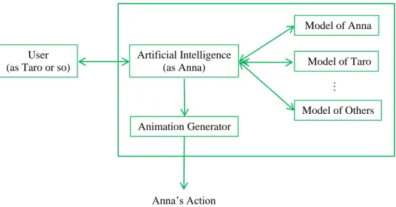
5.3 Conversation Management System... 40
V
TABLE OF CONTENTS
CHAPTER TITLE PAGE
6 Discussion and Conclusion... 67
Appendix A List of Constances……….………... 71
A.1 List of Attribute Constants…………... 71
A.2 List of Standard Constants... 74
A.3 List of Temporal Relations... 75
Appendix B Psycholinguistic Experiment………... 76
B.1 Overview of Psycholinguistic Experiment ... 76
B.2 Type I Sentence…………... 77
B.3 Type II Sentence………….……... 81
B.4 Type III Sentence…... 86
Appendix C List of Word Definitions………... 96
Appendix D CMS source code………... 102
VI
LIST OF FIGURES
FIGURE PAGE
Fig. 1.1 Intuitive thinking process in human... 2
Fig. 1.2 Spatial gestalts………... 2
Fig. 2.1 Loci of the observer’s attention in attribute spaces... 5
Fig. 2.2 Atomic locus... 6
Fig. 2.3 Temporal/spatial change event…... 7
Fig. 2.4 Mental image evoked by the verb “fetch”... 8
Fig. 2.5 Examples of event patterns of physical location... 8
Fig. 2.6 Mental image depiction of S8……... 9
Fig. 2.7 Highly abstract picture of S8……... 9
Fig. 2.8 Highly abstract picture of S9……... 10
Fig. 2.9 Highly abstract picture of S10……... 10
Fig. 3.1 Mental image depiction of S11 and S12... 11
Fig. 3.2 Mental image depiction of S13 and S14... 12
Fig. 3.3 Mental image depiction of S15…... 13
Fig. 3.4 Mental image depiction of S16 and S17... 14
Fig. 3.5 Delicate topological relations: (a) path partially hidden by woods and (b) path winding in-out-in-out of swamp... 15
Fig. 3.6 Bidirectional translation between NL and Lmd via dependency tree... 18
Fig. 3.7 Graphical interpretation of eq. 3.24... 18
Fig. 3.8 Ambiguities in S21... 20
Fig. 4.1 Mental image depiction of S22…... 22
Fig. 5.1 Dependencies possible for S23... 25
Fig 5.2 Highly abstract picture of S23... 25
Fig 5.3 Postulate of continuity in attribute values... 28
VII
LIST OF FIGURES
FIGURE PAGE
Fig 5.5 2nd example of MBU processing for stimulus sentence Type I... 34
Fig 5.6 3rd example of MBU processing for stimulus sentence Type I... 35
Fig 5.7 1st example of MBU processing for stimulus sentence Type II... 36
Fig 5.8 2nd example of MBU processing for stimulus sentence Type II... 37
Fig 5.9 1st example of MBU processing for stimulus sentence Type III... 38
Fig 5.10 2nd example of MBU processing for stimulus sentence Type III... 39
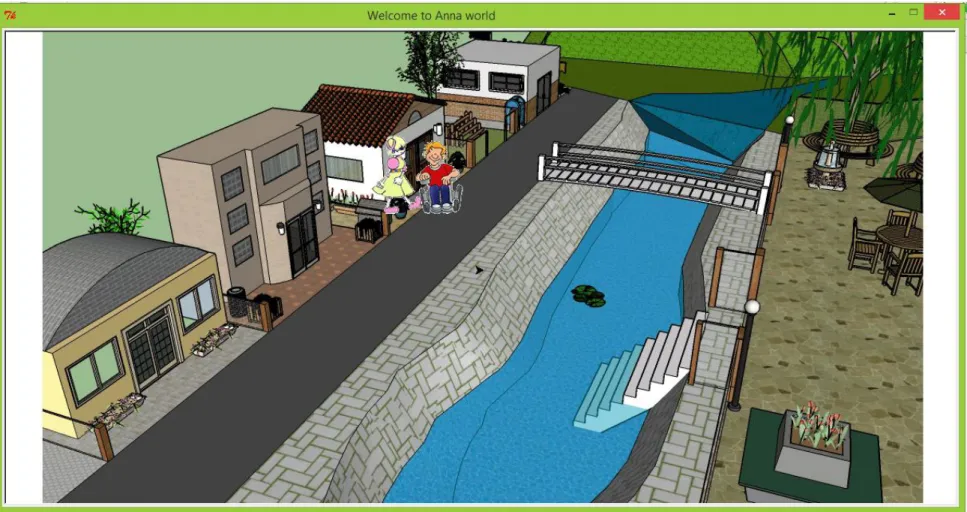
Fig. 5.11 Anna and Taro... 40
Fig 5.12 Conversation management system modules... 41
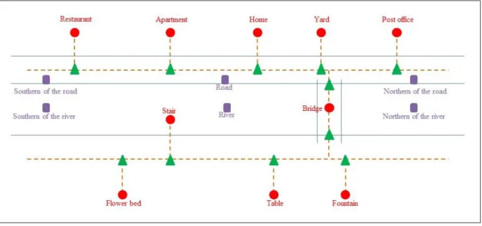
Fig 5.13 Town map in CMS………... 42
Fig 5.14 Graph data of Town map in CMS... 42
Fig 5.15 Anna’s thinking process for S29... 47
Fig 5.16 Translation of Anna’s thinking process for S29... 48
Fig. 5.17 Initial map after the system is executed... 49
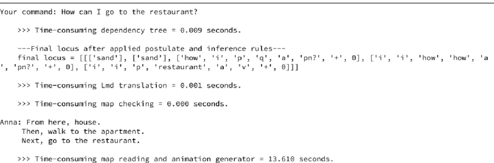
Fig. 5.18 Conversation screen when input is “How can I go to the restaurant?”... 50
Fig. 5.19 Conversation screen when input is “I want to go to the post office”... 51
Fig. 5.20 Changement of animation screen that Taro and Anna move from house to post office.. 52
Fig. 5.21 Conversation screen when input is “Please take me to home”... 53
Fig. 5.22 Changement of animation screen that Taro and Anna move from post office to house.. 54
Fig. 5.23 Conversation screen when input is “When Tom drives to the flower bed with Mary, does she move?”... 55
Fig. 5.24 Tom and Mary are their apartment, before moving to the flower bed... 56
Fig. 5.25 Tom and Mary are the flower bed, after moving from the apartment... 57
Fig. 5.26 Conversation screen when input is “When Tom stays at the flower bed with Mary, does she move?”... 58
VIII
LIST OF FIGURES
FIGURE PAGE
Fig. 5.28 Conversation screen when input is “What is between restaurant and yard?”... 60
Fig. 5.29 Conversation screen when input is “What is between apartment and flower bed?**”... 61
Fig. 5.30 Conversation screen when input is “What is between apartment and flower bed?***”... 62
Fig. 5.31 Conversation screen when input is “I want to call Tom.”... 63
Fig. 5.32 Changement of animation screen after enter input sentence as “I want to call Tom.”… 64
Fig. 5.33 Animation screen changes to house screen, and the phone is on the bed... 65
Fig. 5.34 Anna brings the phone to Taro…... 66
IX
LIST OF TABLES
TABLE PAGE
Table 6.1 Time consuming in Conversation Management System (CMS)... 69
Table A.1 Example of attribute constants in Lmd ... 71
Table A.2 Example of standard constants in Lmd………... 74
Table A.3 Table A.3 List of Temporal relations………... 75
Table B.1. The surveying of Type I stimulus sentence... 77
Table B.2 The surveying of Type II stimulus sentence ... 81
Table B.3 The surveying of Type III stimulus sentence... 86
Table C.1 List of nouns and pronouns………... 96
Table C.2 List of verbs ………...…... 99
Table C.3 List of prepositions ……...……... 100
1
CHAPTER 1
INTRODUCTION
Nowadays, most of our activities always relate to computer equipment. For example, many people use mobile phones for alarm when they wake up and for news reading. Therefore, we cannot refuse that a cell phone is a very basic and useful device that facilitates us not only to contact to each other, but also contains many functions that help us to achieve our desired goals more easily. On the contrary, rapid development of technologies, communications, transportations, and economics has resulted in unnatural and poor social interaction for people. This fact leads to decline of nuptiality and birth rate destined to aging societies. Therefore, many governments are setting policies against these problems. As one of the solutions, robots have come to be widely used items that help people in industrial factories, household sectors and so on. However, these automata will not be able to ease people perfectly, if they lack of smart software called Artificial Intelligence System (AIS), embedded in their organizations.
If we talk about communication methods among people, we may think of many things, for instance, gesture, art, music, etc. Among all, natural language is the most common and convenient method to express our ideas, feeling, thinking, and so forth. In addition, this fact holds as well between man and robot, so called Human-Robot Interaction (HRI).
Reflecting the casual scenes of people and robots, spatiotemporal (4D) language, i.e. language to express topological, directional, metric, and time relations, is the most important to be concerned in order to share knowledge amongst them. 4D language has received special attention in the field of ontology because it includes fundamental issues concerning human cognition such as vagueness and ambiguity. However, traditional approaches have been focused on computing purely objective three-dimension (3D) geometric relations as visual scene [1.1] while people thinking process is often intuitive as shown in Fig. 1.1.
Why can human understand such sentences as S1 – S3 easily? (S1) Tom was on the hill flying a flag back and forth.
(S2) Tom was with the book in the bus running from town to university. (S3) I saw the planet in my room.
2
Along with Fig 1.1 and S1 – S3 expressions, English speakers can experience their understanding about spatial relations as pictures drawn in mind. Therefore, we can recognize objects by mental image. Moreover, we also can cognize and conceive the external world as spatial gestalts shown in Fig. 1.2. That is, human brain is a super marvelous organ!
Fig. 1.1 Intuitive thinking process in human. (S4) Five dots are in line.
(S5) Nine dots are placed in the shape of X.
Fig. 1.2 Spatial gestalts.
Fig. 1.2 (a) and (b) show that human perceives the continuous forms among the dots located separately, and would express them like S4 and S5 respectively.
T. Winograd [1.2] stated that the relationships between Human-Computer Interaction (HCI) and AI for human-like intellect should be described in T-Shaped where horizontal and vertical line were represented to HCI and AI discipline respectively. The famous computer program ELIZA [1.3] is positioned in a very shallow level of this model, that is, doesn’t really understand NL but is designed well to almost pass the Turing test. Then, to test machine intelligence and improve the Turing Test [1.4], Winograd Schema Challenge (WSC) was proposed by H. J. Levesque [1.5] in 2011, and so on [1.6] – [1.7]. Anyway, Natural Language Understanding (NLU) is still one of attractive fields among researchers these days, such as “Watson”, the Q&A cognitive system developed by IBM [1.8] – [1.9]. However, Watson could not understand Natural Language in real sense because it applied Natural Language
(a) (b)
Oh!! I see the moon in the
river.
What is she talking about?? I am too confused.
3
Processing (NLP) techniques to Big Data Analysis. Against this approach, B. M. Lake et al. [1.10] presented the outline in order to build a machine to imitate human learning and thinking processes. Although many works have focused on NLP, it is still extremely difficult to make a machine reach real NLU like people.
This thesis proposes a methodology for natural language understanding (NLU) named Mental-image Based Understanding (MBU), intending that a robot can understand NL as people do. Its application system can reach the most plausible semantic interpretation of an input text and return desirable outcomes based on word concepts, postulates, and inference rules formalized in Mental-image Description Language (Lmd) developed and proposed by M.Yokota in his original theory “Mental Image Directed Semantic Theory (MIDST)” [1.11] - [1.12]. The methodology MBU is implemented in two types of NLU systems named Mental-image Based Understanding System and Conversation Management System. The former is aimed for question-answering with users and the latter performs dialogue management between users and an imaginary robot named Anna. According to our experiments, it has been proved that MBU is simple to use and utilize for semantic interpretation and will be able to influence robots with capability of NLU as well as humans based on a mental image model.
This thesis document consists of 6 chapters that can be summarized as follows. Chapter 1 introduces the background knowledge and the purpose of this work. Chapter 2 describes MIDST to represent human perception process in a computable logical form. Chapter 3 analyzes natural event concepts in association with human attention mechanism from the viewpoint of logical computation. Chapter 4 proposes a problem finding and solving method based on MIDST. Chapter 5 presents Mental-image Based Understanding System and Conversation Management System developed in this work. Finally, chapter 6 discusses and concludes this thesis.
4
CHAPTER 2
PRELIMINARIES
In this chapter, we will introduce Mental Image Directed Semantic Theory (MIDST), a model that we employ to represent human perception process (as shown in Fig. 2.1) in computable logical from, named Language for Mental-Image Description (Lmd) that suitable for “Temporal change events” and “Spatial change events” using attributes of physical objects, and so on.
2.1 Formal System
Formal system is a system that consists of formal language and deductive method where inference rules and postulates are used to derive the theorem. As above mentioned, Lmd is a formal language that employs many-sorted predicate logic with five-kind individual terms specific to the mental image model involved in predicate constant (L), named “Atomic locus” , where the deductive apparatus here is intended to base on deductive system of predicate calculus.
The symbols of the deductive apparatus for Lmd are presented from (i) – (xi) as follows [2.1]. (i) Logical operators: a symbol used to join sentences, i.e. ~, , , ,
(ii) Quantifiers: a symbol used to specify the quantity of instances, i.e. ,
(iii) Meta-symbols: a symbol used to indicate one concept to another concept, i.e. , , , etc.
(iv) Auxiliary constants: a symbol used to qualify or insert into a sentence or passage, i.e. ., (, )
(v) Sentence constant: a symbol used to indicate sentence, i.e. N.
(vi) Predicate constants: a symbol used to indicate predicate, i.e. L, or specify meaning in universal set, e.g. =, ≠, >, <, etc.
(vii) Individual constants: consisting of five types of them: a. Matter constant*
b. Attribute constants: A, B c. Value constant*
d. Pattern constant: G e. Standard constant: K
5
*Please remark that matter and value constant will be introduced when need.
(viii) Function constants: arithmetic operations, e.g. +, - , *, /, etc.
(ix) Sentence variables: a symbol used to represent sub-sentence in sentence constant, i.e. . (x) Individual variables: the variables used to indicate variables in individual constants that
contain of five kinds of terms: a. Matter variable: x, y, z b. Attribute variable: a c. Value variable: p, q, r, s, t d. Pattern variables: g e. Standard variable: k
(xi) Others: a symbol that will be defined by above symbols.
Fig. 2.1 Loci of the observer’s attention in attribute spaces.
Atomic locus or Atomic locus formula is gathered by seven-place predicate that given by eq. 2.1. 𝐿(𝜔1, 𝜔2, 𝜔3, 𝜔4, 𝜔5, 𝜔6, 𝜔7) (eq. 2.1) Where 𝜔1 is a matter as event causer
𝜔2 is a matter as attribute carrier 𝜔3 is a value or matter
𝜔4 is a value or matter 𝜔5 is an attribute of 𝜔2
𝜔6 is a pattern (Temporal or spatial change event) 𝜔7 is a standard or matter
Shape Location
6
In eq. 2.1, 𝜔3, 𝜔4, and 𝜔7 should represent their values over time-interval. Moreover, if 𝜔1,𝜔3, 𝜔4, or 𝜔7 is unknown variable, the symbol “_” can be replaced instead of that variable, while, 𝜔5, the attribute term, can be seen its detail in Appendix A.
However, to simplify eq. 2.1, we can employ variables or constants instead of terms as the following:
𝐿(𝑥, 𝑦, 𝑝, 𝑞, 𝑎, 𝑔, 𝑘) (eq. 2.2) where eq. 2.2 can interpret using Fig 2.2 means that:
“Matter ‘x’ causes Attribute ‘a’ of Matter ‘y’ to keep or change its value temporally or spatially
over a time-interval, where the value ‘p’ and ‘q’ are relative to Standard ‘k’”
Fig. 2.2 Atomic locus.
As above mentioned, Lmd is designed to support for natural event concepts of an attribute in time or space domain (𝑔 𝑖𝑛 𝑒𝑞. 2.2). Therefore, if the event tends to monotonous change/stability over time domain, 𝑔 will be replaced by Temporal change event (𝐺𝑡) . As well as space domain, 𝑔 will be substituted by 𝐺𝑠.
Consider S6 – S7 expressions.
(S6) The train runs from Fukuoka to Kumamoto. (S7) The track runs from Fukuoka to Kumamoto.
S6 and S7 are looked similarly, but when reading these two sentences, we can notice that our eyes (or the Focus of the Attention of the Observer (FAO)) will keep on different objects (or Attribute Carriers (AC)) as show in Fig. 2.3.
Attribute (a) Time (t) 𝑡𝑖 𝑡𝑓 𝑝 𝑞 𝑦 𝑥
7
Fig. 2.3 Temporal/spatial change event.
The green and red arrows in Fig. 2.3 show the differences over time domain. The green one represents the moving train in S6, while the red arrow stands for extended railway from Fukuoka to Kumamoto in S7. So, 𝐺𝑡 and 𝐺𝑠 will supplant 𝑔 in eq. 2.2 respectively. Then, logical form of S6 and S7 can be written as eq. 2.3 and 2.4 severally, when 𝐴12 is physical location.
∃(𝑥, 𝑦, 𝑘)𝐿(𝑥, 𝑦, 𝐹𝑢𝑘𝑢𝑜𝑘𝑎, 𝐾𝑢𝑚𝑎𝑚𝑜𝑡𝑜, 𝐴12, 𝐺𝑡, 𝑘)˄𝑡𝑟𝑎𝑖𝑛(𝑦) (eq. 2.3) ∃(𝑥, 𝑦, 𝑘)𝐿(𝑥, 𝑦, 𝐹𝑢𝑘𝑢𝑜𝑘𝑎, 𝐾𝑢𝑚𝑎𝑚𝑜𝑡𝑜, 𝐴12, 𝐺𝑠, 𝑘)˄𝑡𝑟𝑎𝑐𝑘(𝑦) (eq. 2.4) Normally, when an NL expression is interpreted in Lmd, it always forms of many Atomic Loci. Hence, “Tempo-Logical Connectives (TLCs)”, binary connectives, will be used in deductive system for representing temporal and logical relationships between loci, that is to say “˄” for conjunction, “˅” for disconjunction, “” for implication, and “” for equivalence. Anyway, the most frequently used TLCs in MIDST are “Simultaneous AND” and “Consecutive AND” that can be denoted by “SAND” or “Π” for Simultaneous AND, while “CAND” or “●” are used in place of Consecutive AND.
𝜒1𝐶𝑖𝜒2 (𝜒1𝐶𝜒2)˄𝜏𝑖(𝜒1, 𝜒2) (eq. 2.5) Where, 𝜏−𝑖(𝜒2, 𝜒1) 𝜏𝑖(𝜒1, 𝜒2)(∀𝑖 ∈ {0, ±1, ±2, … , ±6})
Eq. 2.5 is the description of tempo-logical connective 𝐶𝑖, where 𝜒, 𝐶, and 𝜏 refer to a locus, a binary logical connective, and a temporal relation respectively, while 𝑖 is a indexed number. Here, the temporal relation (𝜏) can be divided into thirteen groups by indexed number ranging from -6 to 6 [2.2] (for further details, see APPENDIX A).
Fig. 2.4 illustrates the mental image evoked by the verb fetch, a temporal change event concept, which can be formalized as the locus formula (eq. 2.6) that was detailed in Yokota [2.3]
Temporal change event
Spatial change event
Fukuoka Kumamoto
8
∃(𝑥, 𝑦, 𝑝1, 𝑝2, 𝑘)𝐿(𝑥, 𝑥, 𝑝1, 𝑝2, 𝐴12, 𝐺𝑡, 𝑘) •
𝐿(𝑥, 𝑥, 𝑝2, 𝑝1, 𝐴12, 𝐺𝑡, 𝑘)𝛱𝐿(𝑥, 𝑦, 𝑝2, 𝑝1, 𝐴12, 𝐺𝑡, 𝑘)˄𝑥 ≠ 𝑦𝛬𝑝1≠ 𝑝2 (eq. 2.6)
Fig. 2.4 Mental image evoked by the verb “fetch”.
From all of above, for simplicity in reading and understanding, quantifiers: and will be neglected, and 𝑎, 𝑔, and 𝑘 terms in eq. 2.2 will group them as 𝛼. (See eq. 2.7, where 𝛼 = (𝑎, 𝑔, 𝑘))
𝐿(𝑥, 𝑦, 𝑝, 𝑞, 𝛼) (eq. 2.7) Then, eq. 2.3 and 2.4 can be written in short as follows:
𝐿(_, 𝑡𝑟𝑎𝑖𝑛, 𝐹𝑢𝑘𝑢𝑜𝑘𝑎, 𝐾𝑢𝑚𝑎𝑚𝑜𝑡𝑜, 𝛼𝑡) (eq. 2.8) 𝐿(_, 𝑡𝑟𝑎𝑐𝑘, 𝐹𝑢𝑘𝑢𝑜𝑘𝑎, 𝐾𝑢𝑚𝑎𝑚𝑜𝑡𝑜, 𝛼𝑠) (eq. 2.9) According to the Event Causers in eq. 2.8 and 2.9 are anonymous, so, “_” is employed to place in the first term of these two expressions.
While Fig. 2.5 shows some more examples of event patterns in attribute spaces.
Fig. 2.5 Examples of event patterns of physical location.
x x x x X x x y X y X y X
Return Meet Separate
Carry Start Stop
A12 A12 A12 A12 A12 A12 Time A12 P2 P1 t1 t2 t3 x y
9 2.2 Mental Image Processing
At the topic 2.1, we have described about formal system, the logical expression that is the basic knowledge uses to implement this work. However, in order to make a machine can be aware of NL like people, a methodology that simulate human mental image, Mental-Image Based Understanding (MBU), must be applied. How can this work interpret mental image to Lmd?
Please consider S8:
(S8) The bus runs from Town to University.
Normally, when people read S8 sentence, if we can bring the scene out of our brains, we always think of a moving picture of the running bus that depicted in Fig. 2.6. (Please note that, the words “Town” and “University” in S8 are initialed by capital letters due to bus stop names.)
Fig. 2.6 Mental image depiction of S8.
Anyway, because of immoderate information, so in order to interpret NL expression or image into computable logic, therefore, abstract picture is employed to explain the imagery.
The circle in Fig. 2.7 refers to the object, bus, in S8 expression, while broken arrow is used to represent the movement of the object. Anyhow, please remark that color and shape in the figure are not significant at all.
10 Now please consider S9.
(S9) Tom was with the book in the bus running from Town to University. If applied highly abstract picture to the sentence, what will happen?
Fig. 2.8 Highly abstract picture of S9.
Fig. 2.8 shows the relationships between “Tom”, “Book”, and “Bus” in S9. As above, color and shape are not significant, but if notice, we can see that Tom circle and book circle are touched, what does it mean? The contacting circles mean that “Tom was holding the book by himself”, because the book circle is enclosed by Tom circle. As well as Tom and book circle are also surrounded by bus circle, it implies that “Tom and book were in the bus, while the bus was running from Town to University”.
So, if we ask the S10 to S9, it will not suspect why MBU can return the correct answer as shown in Fig. 2.9.
(S10) Did Tom carry the book from Town to University?
11
CHAPTER 3
FORMULATION OF SUBJECTIVE SPATIOTEMPORAL KNOWLEDGE
AND NATURAL LANGUAGE UNDERSTANDING
Chapter 2 introduced MIDST about its main methodology for mental image formalization. In this chapter, the difference between Spatial and Temporal Change Event is explained based on the relations between Attribute Carrier (AC) and the Focus of the Attention of the Observer (FAO).
3.1 Attribute Carrier and the Focus of the Attention of the Observer
MIDST hypothesizes that the difference between temporal and spatial change event concepts can be attributed to the relationship between the Attribute Carrier (AC) and the Focus of the Attention of the Observer (FAO). To be brief, it is hypothesized that FAO is fixed on the whole AC in a temporal change event but runs about on the AC in a spatial change event. Consequently, the train and FAO move together in the case of S6 while FAO solely moves along the track in the case of S7. That is, all loci in attribute spaces are assumed to correspond one to one with movements or, more generally, temporal change events of FAO.
Therefore, an event expressed in Lmd is compared to a movie film recorded through a floating camera because it is necessarily grounded in FAO’s movement over the event. And this is why S11 and S12 can refer to the same scene in spite of their appearances, where what “sinks” or “rises” is the FAO as illustrated in Fig. 3.1 and whose conceptual descriptions are given as eq. 3.1 and 3.2, respectively.
(S11) The path sinks to the stream. (S12) The path rises from the stream.
Fig. 3.1 Mental image depiction of S11 and S12. FAO
AC
12
𝐿(_, 𝑦, 𝑝, 𝑧, 𝐴12, 𝐺𝑠, _)𝛱𝐿(_, 𝑦, ↓, ↓, 𝐴13, 𝐺𝑠, _)𝛬𝑝𝑎𝑡ℎ(𝑦)𝛬𝑠𝑡𝑟𝑒𝑎𝑚(𝑧)𝛬𝑝 ≠ 𝑧 (eq. 3.1) 𝐿(_, 𝑦, 𝑝, 𝑧, 𝐴12, 𝐺𝑠, _)𝛱𝐿(_, 𝑦, ↑, ↑, 𝐴13, 𝐺𝑠, _)𝛬𝑝𝑎𝑡ℎ(𝑦)𝛬𝑠𝑡𝑟𝑒𝑎𝑚(𝑧)𝛬𝑝 ≠ 𝑧 (eq. 3.2)
Where “A13”, “” and “” in eq. 3.1 and 3.2 refer to the attribute “Direction” and its values
“upward” and “downward”, respectively.
Such a fact is generalized as “Postulate of Reversibility of Spatial Change Event (PRS)”. This postulate is also valid for such a pair of S13 and S14 (depicted as Fig. 3.2) as interpreted approximately into eq. 3.3 and 3.4, respectively. These pairs of conceptual descriptions are called equivalent in the PRS, and the paired sentences are treated as paraphrases each other.
(S13) Route A and Route B meet at the city. (S14) Route A and Route B separate at the city.
Fig. 3.2 Mental image depiction of S13 and S14.
𝐿(_, 𝑅𝑜𝑢𝑡𝑒_𝐴, 𝑝, 𝑦, 𝐴12, 𝐺𝑠, _)𝛱𝐿(_, 𝑅𝑜𝑢𝑡𝑒_𝐵, 𝑞, 𝑦, 𝐴12, 𝐺𝑠, _)𝛬𝑐𝑖𝑡𝑦(𝑦)𝛬𝑝 ≠ 𝑞 (eq. 3.3) 𝐿(_, 𝑅𝑜𝑢𝑡𝑒_𝐴, 𝑦, 𝑝, 𝐴12, 𝐺𝑠, _)𝛱𝐿(_, 𝑅𝑜𝑢𝑡𝑒_𝐵, 𝑦, 𝑞, 𝐴12, 𝐺𝑠, _)𝛬𝑐𝑖𝑡𝑦(𝑦)𝛬𝑝 ≠ 𝑞 (eq. 3.4) For another example of Spatial Change Event, please consider S15 that Fig. 3.3 concerns the perception of the formation of multiple objects, where FAO runs along an imaginary object so called “Imaginary Space Region (ISR)”.
p q
13
(S15) The square is between the triangle and the circle.
(𝐿(_, 𝑦, 𝑥1, 𝑥2, 𝐴12, 𝐺𝑠, _)𝛱𝐿(_, 𝑦, 𝑝, 𝑝, 𝐴13, 𝐺𝑠, _))
●(𝐿(_, 𝑦, 𝑥2, 𝑥3, 𝐴12, 𝐺𝑠, _)𝛱𝐿(_, 𝑦, 𝑞, 𝑞, 𝐴13, 𝐺𝑠, _))𝛬𝐼𝑆𝑅(𝑦)
𝛬𝑝 = 𝑞𝛬𝑡𝑟𝑖𝑎𝑛𝑔𝑙𝑒(𝑥1)𝛬𝑠𝑞𝑢𝑎𝑟𝑒(𝑥2)𝛬𝑐𝑖𝑟𝑐𝑙𝑒(𝑥3) (eq. 3.5)
Fig. 3.3 Mental image depiction of S15.
Fig. 3.3 is mental image of S15 that preposition “between” is used and formulated as eq. 3.5 or eq. 3.6, corresponding also to such concepts as “row”, “line-up”, etc.
(𝐿(_, 𝑦, 𝑥1, 𝑥2, 𝐴12, 𝐺𝑠, _)●(𝐿(_, 𝑦, 𝑥2, 𝑥3, 𝐴12, 𝐺𝑠, _))
𝛱𝐿(_, 𝑦, 𝑝, 𝑝, 𝐴13, 𝐺𝑠, _))𝛬𝐼𝑆𝑅(𝑦)𝛬𝑡𝑟𝑖𝑎𝑛𝑔𝑙𝑒(𝑥1)𝛬𝑠𝑞𝑢𝑎𝑟𝑒(𝑥2)𝛬𝑐𝑖𝑟𝑐𝑙𝑒(𝑥3) (eq. 3.6) In order to employ ISRs and the 9 - intersection model [3.1], topological relations between two objects can be formulated in such expressions, S16 and S17.
(S16) Tom is in the room.
𝐿(𝑇𝑜𝑚, 𝑥, 𝑦, 𝑇𝑜𝑚, 𝐴12, 𝐺𝑠, _)𝛱𝐿(𝑇𝑜𝑚, 𝑥, 𝐼𝑛, 𝐼𝑛, 𝐴44, 𝐺𝑡, 𝐾9𝐼𝑀)𝛬𝐼𝑆𝑅(𝑥)𝛬𝑟𝑜𝑜𝑚(𝑦) (eq. 3.7) 𝐿(𝑇𝑜𝑚, 𝑥, 𝑇𝑜𝑚, 𝑦, 𝐴12, 𝐺𝑠, _)𝛱𝐿(𝑇𝑜𝑚, 𝑥, 𝐶𝑜𝑛𝑡, 𝐶𝑜𝑛𝑡, 𝐴44, 𝐺𝑡, 𝐾9𝐼𝑀)𝛬𝐼𝑆𝑅(𝑥)𝛬𝑟𝑜𝑜𝑚(𝑦) (eq. 3.8)
(S17) Tom exits the room.
𝐿(𝑇𝑜𝑚, 𝑇𝑜𝑚, 𝑝, 𝑞, 𝐴12, 𝐺𝑡, _)𝛱𝐿(𝑇𝑜𝑚, 𝑥, 𝑦, 𝑇𝑜𝑚, 𝐴12, 𝐺𝑠, _)
𝛱𝐿(𝑇𝑜𝑚, 𝑥, 𝐼𝑛, 𝐷𝑖𝑠, 𝐴44, 𝐺𝑡, 𝐾9𝐼𝑀)𝛬𝐼𝑆𝑅(𝑥)𝛬𝑟𝑜𝑜𝑚(𝑦)𝛬𝑝 ≠ 𝑞 (eq. 3.9)
FAO
14
Fig. 3.4 Mental image depiction of S16 and S17.
From above, eq. 3.7 and eq. 3.8 represent Lmd expression of S16, while eq. 3.9 is the interpretation of S17, where “In”, “Cont” and “Dis” refer to “inside”, “contains” and “disjoint” of the attribute “Topology (A44)” with the standard “9 - intersection model (K9IM)”, respectively. Please remark that,
these topological values are given as 33 matrices with each element equal to 0 or 1 and therefore, for example, “In” and “Cont” are transposes each other.
The mathematically rigid topology between two objects must be determined with the perfect knowledge of their insides, outsides and boundaries [3.1]. Ordinary people, however, would often comment on matters without knowing all about them. This is the very case when they encounter an unknown object too large to observe at a glance just like a road in a strange country.
For example, Fig. 3.5(a) shows bird’s-eye view of a path that is partly hidden by woods.
15
Fig. 3.5 Delicate topological relations:
(a) path partially hidden by woods and (b) path winding in-out-in-out of swamp.
In this case, the topological relation between the path as a whole and the swamp/woods depends on how the path starts and ends in the woods, but people could utter such sentences as S18 and S19 about this scene. Actually, these sentences refer to such events that reflect certain temporal changes in the topological relation between the swamp/woods and the FAO running along the path.
(S18) The path goes into the swamp/woods. (S19) The path comes out of the swamp/woods.
Therefore, their conceptual descriptions are to be given as eq. 3.10 and eq. 3.11, respectively. 𝐿(_, 𝑧, 𝑝, 𝑞, 𝐴12, 𝐺𝑠, _)𝛱𝐿(_, 𝑥, 𝑦, 𝑧, 𝐴12, 𝐺𝑠, _) 𝛱𝐿(_, 𝑥, 𝐷𝑖𝑠, 𝐼𝑛, 𝐴44, 𝐺𝑠, 𝐾9𝐼𝑀)𝛬𝐼𝑆𝑅(𝑥) 𝛬{𝑠𝑤𝑎𝑚𝑝(𝑦)/𝑤𝑜𝑜𝑑𝑠(𝑦)}𝛬𝑝𝑎𝑡ℎ(𝑧)𝛬𝑝 ≠ 𝑞 (eq. 3.10) 𝐿(_, 𝑧, 𝑝, 𝑞, 𝐴12, 𝐺𝑠, _)𝛱𝐿(_, 𝑥, 𝑦, 𝑧, 𝐴12, 𝐺𝑠, _) 𝛱𝐿(_, 𝑥, 𝐼𝑛, 𝐷𝑖𝑠, 𝐴44, 𝐺𝑠, 𝐾9𝐼𝑀)𝛬𝐼𝑆𝑅(𝑥) 𝛬{𝑠𝑤𝑎𝑚𝑝(𝑦)/𝑤𝑜𝑜𝑑𝑠(𝑦)}𝛬𝑝𝑎𝑡ℎ(𝑧)𝛬𝑝 ≠ 𝑞 (eq. 3.11)
For another example, Fig. 3.5(b), a portrayed image of S20, shows a more complicated spatial event in topology that can be formulated as eq. 3.12.
16 𝐿(_, 𝑧, 𝑦, 𝑥, 𝐴12, 𝐺𝑠, _)𝛱((𝐿(_, 𝑥, 𝑝1, 𝑝2, 𝐴12, 𝐺𝑠, _)𝛱(𝐿(_, 𝑧, 𝐷𝑖𝑠, 𝐼𝑛, 𝐴44, 𝐺𝑠, 𝐾9𝐼𝑀)) ●(𝐿(_, 𝑥, 𝑝2, 𝑝3, 𝐴12, 𝐺𝑠, _)𝛱𝐿(_, 𝑧, 𝐼𝑛, 𝐷𝑖𝑠, 𝐴44, 𝐺𝑠, 𝐾9𝐼𝑀)) ●(𝐿(_, 𝑥, 𝑝3, 𝑝4, 𝐴12, 𝐺𝑠, _)𝛱𝐿(_, 𝑧, 𝐷𝑖𝑠, 𝐼𝑛, 𝐴44, 𝐺𝑠, 𝐾9𝐼𝑀)) ●(𝐿(,𝑥, 𝑝4, 𝑝5, 𝐴12, 𝐺𝑠, _)𝛱𝐿(,𝑧, 𝐼𝑛, 𝐷𝑖𝑠, 𝐴44, 𝐺𝑠, 𝐾9𝐼𝑀))) 𝛬𝑝𝑎𝑡ℎ(𝑥)𝛬𝑠𝑤𝑎𝑚𝑝(𝑦)𝛬𝐼𝑆𝑅(𝑧) (eq. 3.12)
Conventional approaches to spatial or 3D language understanding have inevitably employed a tremendously great number of axioms such as eq. 3.13. It is noticeable that these axioms are part of the definition of “between” valid only for verbalized directions such as “left” and “above” and that actually much more axioms should be needed for other directions such as “before” and “behind”.
𝑟𝑖𝑔ℎ𝑡(𝑥, 𝑦) ≡ 𝑙𝑒𝑓𝑡(𝑦, 𝑥) 𝑎𝑏𝑜𝑣𝑒(𝑥, 𝑦) ≡ 𝑢𝑛𝑑𝑒𝑟(𝑦, 𝑥)
𝑎𝑏𝑜𝑣𝑒(𝑦, 𝑥)&𝑎𝑏𝑜𝑣𝑒(𝑥, 𝑧) 𝑏𝑒𝑡𝑤𝑒𝑒𝑛(𝑥, 𝑦, 𝑧)
𝑟𝑖𝑔ℎ𝑡(𝑦, 𝑥)&𝑟𝑖𝑔ℎ𝑡(𝑥, 𝑧) 𝑏𝑒𝑡𝑤𝑒𝑒𝑛(𝑥, 𝑦, 𝑧) (eq. 3.13)
Distinguishably, MIDST gives the definition of “between” in such a simple and language-free formula as the underlined part of eq. 3.14 (as same as eq. 3.6) and moreover that is applicable to every direction, whether or not verbalized. The concepts of 40 English prepositions, so-called, spatial prepositions such as “along” were analyzed and formulated in accordance with MIDST. To be most remarkable, the concepts of spatial prepositions are defined as 4D images in MIDST but not as 3D (i.e. 4D exclude “time”) images in conventional approaches.
(𝐿(_, 𝑦, 𝑥1, 𝑥2, 𝐴12, 𝐺𝑠, _)●(𝐿(_, 𝑦, 𝑥2, 𝑥3, 𝐴12, 𝐺𝑠, _)) 𝛱𝐿(_, 𝑦, 𝑝, 𝑝, 𝐴13, 𝐺𝑠, _))𝛬𝐼𝑆𝑅(𝑦)
𝛬𝑡𝑟𝑖𝑎𝑛𝑔𝑙𝑒(𝑥1)𝛬𝑠𝑞𝑢𝑎𝑟𝑒(𝑥2)𝛬𝑐𝑖𝑟𝑐𝑙𝑒(𝑥3) (eq. 3.14)
3.2 Translation Process between Natural Language Expression and Lmd
Natural language and Lmd are translated into each other via dependency tree employed in conventional natural language processing for grammatical description. The bidirectional translation between dependency tree and Lmd is operated by mapping rules assigned to functional words such as verbs and prepositions indicating how their context in NL should be mapped into or generated from the counterpart in Lmd. Here, the mapping rule of a word W is generalized as eq. 3.15.
17
𝐶𝑜𝑛𝑡𝑒𝑥𝑡 𝑔𝑜𝑣𝑒𝑟𝑛𝑒𝑑 𝑏𝑦 𝑊 𝐶𝑜𝑛𝑐𝑒𝑝𝑡 𝑜𝑓 𝑊 𝑖𝑛 𝑳𝒎𝒅 (eq. 3.15)
For example, the mapping rules of “with”, “at”, “move”, “carry”, “run”, “take” and “bring back” are given by eq. 3.16 – eq. 3.24, where Ʌ𝑡 = (𝐴12, 𝐺𝑡, 𝑘) and Ʌ𝑠= (𝐴12, 𝐺𝑠, 𝑘). Hereafter, for the sake of simplicity, explicit indications of the quantifiers (i.e., ∀ and ∃) and the relations among variables (e.g., 𝑥 𝑦) are often omitted without risk of confusion.
𝑥 (𝑏𝑒) 𝑤𝑖𝑡ℎ 𝑦 𝐿(𝑥, 𝑦, 𝑥, 𝑥, Ʌ𝑡) (eq. 3.16) 𝑥 (𝑏𝑒) 𝑎𝑡 𝑦 𝐿(𝑥, 𝑥, 𝑦, 𝑥, Ʌ𝑡) (eq. 3.17) 𝑥 𝑚𝑜𝑣𝑒 𝑦 𝑓𝑟𝑜𝑚 𝑝 𝑡𝑜 𝑞 𝐿(𝑥, 𝑦, 𝑝, 𝑞, Ʌ𝑡) (eq. 3.18) 𝑥 𝑐𝑎𝑟𝑟𝑦1 𝑦 𝑓𝑟𝑜𝑚 𝑝 𝑡𝑜 𝑞 𝐿(𝑥, 𝑥, 𝑝, 𝑞, Ʌ 𝑡)𝛱𝐿(𝑥, 𝑦, 𝑝, 𝑞, Ʌ𝑡) (eq. 3.19) 𝑥 𝑐𝑎𝑟𝑟𝑦2 𝑦 𝑓𝑟𝑜𝑚 𝑝 𝑡𝑜 𝑞 𝐿(𝑥, 𝑦, 𝑥, 𝑥, Ʌ𝑡)𝛱𝐿(𝑥, 𝑥, 𝑝, 𝑞, Ʌ𝑡) (eq. 3.20)
𝑥 𝑟𝑢𝑛 𝑓𝑟𝑜𝑚 𝑝 𝑡𝑜 𝑞 𝐿(𝑥, 𝑥, 𝑝, 𝑞, Ʌ𝑡) (Temporal Change Event) (eq. 3.21)
𝑥 𝑟𝑢𝑛 𝑓𝑟𝑜𝑚 𝑝 𝑡𝑜 𝑞 𝐿(𝑥, 𝑥, 𝑝, 𝑞, Ʌ𝑠) (Spatial Change Event) (eq. 3.22)
𝑥 𝑡𝑎𝑘𝑒 𝑦 𝑓𝑟𝑜𝑚 𝑧 𝐿(𝑥, 𝑦, 𝑧, 𝑥, Ʌ𝑡) (eq. 3.23)
𝑥 𝑏𝑟𝑖𝑛𝑔 𝑏𝑎𝑐𝑘 𝑦 𝑡𝑜 𝑝 𝑓𝑟𝑜𝑚 𝑞 𝐿(𝑥, 𝑥, 𝑝, 𝑞, Ʌ𝑡)●𝜒 ●(𝐿(𝑥, 𝑦, 𝑥, 𝑥, Ʌ𝑡)𝛱𝐿(𝑥, 𝑥, 𝑞, 𝑝, Ʌ𝑡))
(where χ is an Lmd expression) (eq. 3.24) 1,2 Please remark that, “carry” can be defined in the two ways as shown in eq. 3.19 and eq. 3.20.
18 Consider to interpret S20 in Lmd.
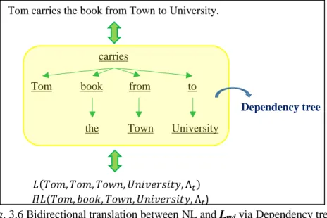
(S20) Tom carries the book from Town to University.
Fig. 3.6 Bidirectional translation between NL and Lmd via Dependency tree.
Fig. 3.6 shows the bidirectional translation between S20 and its semantic interpretation (eq. 3.25) via the dependency tree formulated as eq. 3.26.
𝐿(𝑇𝑜𝑚, 𝑇𝑜𝑚, 𝑇𝑜𝑤𝑛, 𝑈𝑛𝑖𝑣𝑒𝑟𝑠𝑖𝑡𝑦, Ʌ𝑡)𝛱𝐿(𝑇𝑜𝑚, 𝑏𝑜𝑜𝑘, 𝑇𝑜𝑤𝑛, 𝑈𝑛𝑖𝑣𝑒𝑟𝑠𝑖𝑡𝑦, Ʌ𝑡) (eq. 3.25)
𝑐𝑎𝑟𝑟𝑖𝑒𝑠(𝑇𝑜𝑚, 𝑏𝑜𝑜𝑘(𝑡ℎ𝑒), 𝑓𝑟𝑜𝑚(𝑇𝑜𝑤𝑛), 𝑡𝑜(𝑈𝑛𝑖𝑣𝑒𝑟𝑠𝑖𝑡𝑦)) (eq. 3.26)
The formula eq. 3.24 reads “Tom moves from Town to University by himself and simultaneously () Tom moves the book from Town to University” and it can be depicted as Fig. 3.7.
Fig. 3.7 Graphical interpretation of eq. 3.24. Tom carries the book from Town to University.
carries
Tom book from to
the Town University
𝐿(𝑇𝑜𝑚, 𝑇𝑜𝑚, 𝑇𝑜𝑤𝑛, 𝑈𝑛𝑖𝑣𝑒𝑟𝑠𝑖𝑡𝑦, Ʌ𝑡) 𝛱𝐿(𝑇𝑜𝑚, 𝑏𝑜𝑜𝑘, 𝑇𝑜𝑤𝑛, 𝑈𝑛𝑖𝑣𝑒𝑟𝑠𝑖𝑡𝑦, Ʌ𝑡) Dependency tree A12 Time University Town book Tom
19 3.3 Evaluation of Semantic Interpretation
Such a semantic interpretation as eq. 3.25 is to be evaluated about its plausibility. For this purpose, entity word concepts such as “cat” and “car” are exclusively utilized. The concept of an entity can be defined as a set of locus formulas representing its potentiality at every attribute. For example, “Tom”, “book” and “hill” can be defined as eq. 3.27 – eq. 3.29 at the attribute “Physical Location (A12)” with 𝑔 =
𝐺𝑡, where the symbol + or denotes whether the following image is positive (i.e., probable) or negative (i.e., improbable), respectively.
{+𝐿(𝑇𝑜𝑚, 𝑇𝑜𝑚, 𝑝, 𝑞, Ʌ𝑡), +𝐿(𝑇𝑜𝑚, 𝑥, 𝑝, 𝑞, Ʌ𝑡), … } (eq. 3.27) {−𝐿(𝐵𝑜𝑜𝑘, 𝐵𝑜𝑜𝑘, 𝑝, 𝑞, Ʌ𝑡), +𝐿(𝑦, 𝐵𝑜𝑜𝑘, 𝑝, 𝑞, Ʌ𝑡), … } (eq. 3.28) {−𝐿(𝑧, 𝐻𝑖𝑙𝑙, 𝑝, 𝑞, Ʌ𝑡), −𝐿(𝐻𝑖𝑙𝑙, 𝑧, 𝑝, 𝑞, Ʌ𝑡), … } (eq. 3.29) The meaning of each formula in these is as follows.
+𝐿(𝑇𝑜𝑚, 𝑇𝑜𝑚, 𝑝, 𝑞, Ʌ𝑡): “Tom moves by himself” is probable. +𝐿(𝑇𝑜𝑚, 𝑥, 𝑝, 𝑞, Ʌ𝑡): “Tom moves something” is probable. −𝐿(𝐵𝑜𝑜𝑘, 𝐵𝑜𝑜𝑘, 𝑝, 𝑞, Ʌ𝑡): “A book moves itself” is improbable. +𝐿(𝑦, 𝐵𝑜𝑜𝑘, 𝑝, 𝑞, Ʌ𝑡): “A book is moved” is probable. −𝐿(𝑧, 𝐻𝑖𝑙𝑙, 𝑝, 𝑞, Ʌ𝑡): “A hill is moved” is improbable.
−𝐿(𝐻𝑖𝑙𝑙, 𝑧, 𝑝, 𝑞, Ʌ𝑡): “A hill moves something” is improbable.
The definitions of “Tom” and “book” do not conflict with eq. 3.25 and therefore the semantic interpretation of S20 proves to be plausible. For another example, consider S21.
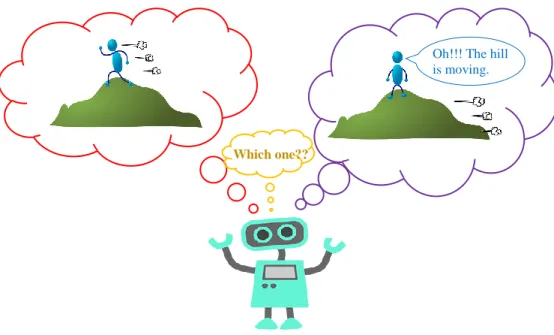
(S21) Tom was on the hill, moving about.
This sentence is syntactically ambiguous in two ways as shown in Fig. 3.8, that is, both “Tom” and “hill” can be the subject of “moving” grammatically. However, “Tom” is more plausible because “Tom moves (by himself)” is probable but “a hill moves” is improbable.
20
Fig. 3.8 Ambiguities in S21
For the semantic evaluation described above, a simple pattern matching operation (PMO), so-called unification in conventional AI, is employed to search one Lmd expression such as eq. 3.25 for another Lmd expression such as the underlined part of eq. 3.27. This kind of semantic evaluation can prevent cognitive robots from meaningless and endless work due to such an anomalous command as S21 given by mischievous people.
Oh!!! The hill is moving.
21
CHAPTER 4
PROBLEM FINDING AND SOLVING IN L
mdThis section is about problem finding and solving method in this work, consisting of “definition of problem and task”, “creation of problem finding and solving”, and “maintenance problem finding and solving”, respectively.
Imagine such a scene that a robot is working in order to achieve its mission assigned by some people. The robot must find and solve problems concerning the mission. The problems here are considered to belong to the category Exploration problem introduced in Heylighen [4.1] for robots partially or wholly ignorant of their environments. Such problems can be classified roughly into two subcategories as follows.
Creation Problem (PC): house building, food cooking, etc.
Maintenance Problem (PM): fire extinguishing, room cleaning, etc.
In general, a PM is relatively simple one that the robot can find and solve autonomously while a
PC is relatively difficult one that is given to the robot, possibly, by humans and to be solved in
cooperation with them.
4.1 Definition of Problem and Task
The robot must determine its task to solve a problem in the world. In general, during such problem solving, the robot needs to interpolate some transit event 𝑋𝑇between the two events, namely,
Current Event (𝑋𝐶) and Goal Event (𝑋𝐺) as shown by (eq. 4.1).
𝑋𝐶●𝑋𝑇●𝑋𝐺 (eq. 4.1) According to this formalization, a problem 𝑋𝑃 is defined as 𝑋𝑇𝑋𝐺 and a task for the robot is defined as its realization in the same way as the conventional AI referred to by Russell and Norvig [4.2], etc., where a problem is defined as the difference or gap between a Current State and a Goal State and a task as its cancellation. Here, the term Event is preferred to the term State, and instead State is defined as static Event which corresponds to a level locus. The events in the world are described as loci in certain attribute spaces and a problem is to be detected by the unit of atomic locus as event gaps. For example,
22
employing such a postulate of Continuity in attribute values (PCAV), the event gap 𝑋 in (eq. 4.2) is to be
inferred as (eq. 4.3).
𝐿(𝑥, 𝑦, 𝑞1, 𝑞2, 𝑎, 𝑔, 𝑘)●𝑋●𝐿(𝑧, 𝑦, 𝑞3, 𝑞4, 𝑎, 𝑔, 𝑘) (eq. 4.2) 𝐿(𝑧′, 𝑦, 𝑞2, 𝑞3, 𝑎, 𝑔, 𝑘) (eq. 4.3)
4.2 Creation Problem Finding and Solving
Consider such a verbal command as S22 uttered by a human. Its interpretation is given by (eq. 4.4) as the goal event 𝑋𝐺 concerning the attribute, Height (A03). If the current event 𝑋𝐶 is given by (eq. 4.5), then (eq. 4.6) with the transit event 𝑋𝑇 underlined can be inferred as the problem corresponding to S22.
(S22) Keep balloon 𝐶7 flying 7-9 meters high.
Fig. 4.1 Mental image depiction of S22.
𝐿(𝑧, 𝐶7, 𝑞, 𝑞, 𝐴03, 𝐺𝑡, 𝑘)●𝑏𝑎𝑙𝑙𝑜𝑜𝑛(𝐶7)Ʌ7𝑚 ≤ 𝑞 ≤ 9𝑚 (eq. 4.4) 𝐿(𝑥, 𝐶7, 𝑝, 𝑝, 𝐴03, 𝐺𝑡, 𝑘)Ʌ𝑏𝑎𝑙𝑙𝑜𝑜𝑛(𝐶7) (eq. 4.5) 𝐿(𝑧1, 𝐶7, 𝑝, 𝑞, 𝐴03, 𝐺𝑡, 𝑘)●𝐿(𝑧, 𝐶7, 𝑞, 𝑞, 𝐴03, 𝐺𝑡, 𝑘)
Ʌ𝑏𝑎𝑙𝑙𝑜𝑜𝑛(𝐶7)Ʌ7𝑚 ≤ 𝑞 ≤ 9𝑚 (eq. 4.6) 7 - 9 Meters
23
For this problem, the robot is to execute a task deploying a certain height sensor and actors, z1 and
z. The selection of the actor z1 is performed as follows:
If 9m-p <0 then z1 is a sinker, otherwise
if 7m-p >0 then z1 is a raiser, otherwise
7mp9m and no actor is deployed as z1.
The selection of z is a task in case of PM described below.
4.3 Maintenance Problem Finding and Solving
In general, the goal event 𝑋𝐺 for a 𝑃𝑀 is that for another 𝑃𝐶 such as S22 given possibly by humans and solved by the robot in advance. That is, the task in this case is to autonomously restore the goal event 𝑋𝐺 created in advance to the current event 𝑋𝐶 as shown in eq. 4.7, where the transit event 𝑋𝑇 is the reversal of such 𝑋−𝑇that has been already detected as abnormal by the robot.
For example, if 𝑋𝐺 is given by eq. 4.4 in advance, 𝑋𝑇 is also represented as the underlined part of eq. 4.6 while 𝑋−𝑇as eq. 4.8. Therefore the task here is quite the same that was described in the previous subsection 4.2.
𝑋𝐺●𝑋−𝑇●𝑋𝐶●𝑋𝑇●𝑋𝐺 (eq. 4.7) 𝐿(𝑧1, 𝐶7, 𝑞, 𝑝, 𝐴03, 𝐺𝑡, 𝑘)Ʌ𝑏𝑎𝑙𝑙𝑜𝑜𝑛(𝐶7) (eq. 4.8)
24
CHAPTER 5
APPLICATIONS TO NATURAL LANGUAGE UNDERSTANDING
In this work, we have been developing a Mental – Image Based Understanding system (MBU) and Conversation Management System (CMS) in Python for simulating human-robot interaction in NL [5.1] that the details are as the following.
5.1 Mental – Image Based Understanding
Mental – Image Based Understanding (MBU) is a system based on MIDST to simulate human mental imagery, focusing on 4D expressions to obtain the results in an acceptable way (like Q&A) where mental images are represented by the formal language Lmd.
For this work on MBU, Lmd was applied to three types of stimulus sentences as follows, where SS, PrP, PaP and C denote “simple sentence”, “present particle construction”, “past particle construction” and “conjunction”, respectively.
[Type I] Simple sentence + Present particle construction (SS + PrP) For example:
(S23) Tom was with the book in the bus running from Town to University. (= S9) [Type II] Simple sentence + Past particle construction (SS + PaP)
For example:
(S24) Tom was with the book in the car driven from Town to University by Mary. [Type III] Simple sentence + Conjunction + Simple sentence (SS + C + SS)
For example:
(S25) Tom kept the book in a box before he drove the car from Town to University with the box.
As easily convinced, S23 – S25 are syntactically ambiguous that may be rather easy for humans to understand, but it is not the case for robots.
25
For example, consider S23. How can the machine know who/what was running from Town to University? —Tom, or book, or bus? Here, to see its syntactic possibilities, Dependency Grammar (DG) is employed to determine the relations between head words and their dependents. In principle, S23 can have twelve possible dependency trees, that is, syntactically ambiguous in twelve ways as shown in Fig.5.1. This can be formulated by a set of local dependencies such as eq. 5.1, where each pair of parentheses is for the alternatives causing the syntactic ambiguity.
Fig. 5.1 Dependencies possible for S23.
{𝐷11, 𝐷12, (𝐷13|𝐷13𝑎), (𝐷21|𝐷21𝑎|𝐷21𝑏), 𝐷22, (𝐷23|𝐷23𝑎)} (eq. 5.1) According to our psychological experiment, almost all the human subjects reach very easily the most plausible image (i.e., Fig. 5.2) that corresponds directly to the dependency tree defined by eq. 5.2 and can be formulated as eq. 5.3 in Lmd.
Fig 5.2 Highly abstract picture of S23.
{𝐷11, 𝐷12, 𝐷13, 𝐷21, 𝐷22, 𝐷23} (eq. 5.2) 𝐿(𝑇𝑜𝑚, 𝐵𝑜𝑜𝑘, 𝑇𝑜𝑚, 𝑇𝑜𝑚, 𝛬𝑡)𝛱𝐿(𝑧, 𝑇𝑜𝑚, 𝐵𝑢𝑠, 𝐵𝑢𝑠, 𝛬𝑡) 𝛱𝐿(𝐵𝑢𝑠, 𝐵𝑢𝑠, 𝑇𝑜𝑤𝑛, 𝑈𝑛𝑖𝑣. , 𝛬𝑡) (eq. 5.3)
was
Tom with the in the bus
runnin
from Town to University
D11 D12 D13 D13a D21b D21a D21 D22 D23 D23a
26
Quite in the same way, the most plausible interpretations of S24 and S25 are given by eq. 5.4 and eq. 5.5, respectively.
𝐿(𝑇𝑜𝑚, 𝐵𝑜𝑜𝑘, 𝑇𝑜𝑚, 𝑇𝑜𝑚, 𝛬𝑡)𝛱𝐿(𝑧, 𝑇𝑜𝑚, 𝐶𝑎𝑟, 𝐶𝑎𝑟, 𝛬𝑡) 𝛱𝐿(𝑀𝑎𝑟𝑦, 𝑀𝑎𝑟𝑦, 𝐶𝑎𝑟, 𝐶𝑎𝑟, 𝛬𝑡)𝛱𝐿(𝑀𝑎𝑟𝑦, 𝐶𝑎𝑟, 𝑇𝑜𝑤𝑛, 𝑈𝑛𝑖𝑣. , 𝛬𝑡) (eq. 5.4)
𝐿(𝑇𝑜𝑚, 𝐵𝑜𝑜𝑘, 𝐵𝑜𝑥, 𝐵𝑜𝑥, 𝛬𝑡)●(𝐿(𝑇𝑜𝑚, 𝑇𝑜𝑚, 𝐶𝑎𝑟, 𝐶𝑎𝑟, 𝛬𝑡) 𝛱𝐿(𝑇𝑜𝑚, 𝐶𝑎𝑟, 𝑇𝑜𝑤𝑛, 𝑈𝑛𝑖𝑣. , 𝛬𝑡)𝛱𝐿(𝑇𝑜𝑚, 𝐵𝑜𝑥, 𝑇𝑜𝑚, 𝑇𝑜𝑚, 𝛬𝑡)) (eq. 5.5)
Every semantic interpretation (e.g., eq. 5.3) of an NL expression (i.e., S23) is generated by unifying the word meanings according to its corresponding dependency tree (i.e., eq. 5.2). In this process, functional words such as verbs and prepositions are employed for structuring the locus formulas, such as eq. 5.6 – 5.7 (for more example, see section 3.2, Translation process between Natural Language expression and Lmd)
𝑥 𝑑𝑟𝑖𝑣𝑒𝑠 𝑦 𝑓𝑟𝑜𝑚 𝑝 𝑡𝑜 𝑞 𝐿(𝑥, 𝑥, 𝑦, 𝑦, Ʌ𝑡)𝛱𝐿(𝑥, 𝑦, 𝑝, 𝑞, Ʌ𝑡) (eq. 5.6) 𝑥 𝑘𝑒𝑒𝑝𝑠 𝑦 𝑖𝑛 𝑧 𝐿(𝑥, 𝑦, 𝑧, 𝑧, Ʌ𝑡) (eq. 5.7) On the other hand, entity names such as “Tom”, “book” and “bus” are non-functional but utilized for disambiguation in syntactic dependency. Our psychological experiment (for more information, see APPENDIX B) revealed that the subjects remembered their own experiences in association with the entity names and that they selected the dependency corresponding to their most familiar experience among all the possibilities (The detail of disambiguation process is described in section 3.3, Evaluation of Semantic Interpretation).
{+𝐿(𝐵𝑢𝑠, 𝐵𝑢𝑠, 𝑝, 𝑞, Ʌ𝑡), +𝐿(𝐵𝑢𝑠, 𝑥, 𝑝, 𝑞, Ʌ𝑡), +𝐿(𝑥, 𝐻𝑢𝑚𝑎𝑛, 𝐵𝑢𝑠, 𝐵𝑢𝑠, Ʌ𝑡), … } (eq. 5.8) It is sure that the subjects reached the most plausible interpretation eq. 5.3 almost unconsciously by using these evoked images for disambiguation. For example, the image for D13 in Fig. 5.1 is more probable than that for D13a because of eq. 3.26 and eq. 5.8, D21b is improbable because of eq. 3.27, and the combination of D13 and D21a results in somewhat strange image that Tom was running in the bus, and therefore D21a is seldom selected.
Furthermore, as well as disambiguation, question - answering in MBU was simulated, which is performed by “Pattern Matching (PM)” between the locus formulas of an assertion and a question, for example, eq. 5.3 of S23 and eq. 5.9 of S26.
27
(S26) Did Tom carry the book from Town to University?
𝐿(𝑧, 𝐵𝑜𝑜𝑘, 𝑇𝑜𝑚, 𝑇𝑜𝑚, 𝛬𝑡)𝛱𝐿(𝑇𝑜𝑚, 𝑇𝑜𝑚, 𝑇𝑜𝑤𝑛, 𝑈𝑛𝑖𝑣. , 𝛬𝑡) (eq. 5.9) Actually, “carry” is defined in the two ways as eq. 3.19 and eq. 3.20 but, from now on, only either
of them is considered for the sake of simplicity. For example, eq. 5.9 adopts eq. 3.20.
If eq. 5.3 includes eq. 5.9 as is, the answer is positive, but this is not the case. That is, direct trial of PM to the locus formulas eq. 5.3 – eq. 5.5 does not always lead to the desirable outcomes. Therefore, a number of postulates and inference rules must be introduced. The postulates such as P1 – P4 are formulas representing pieces of people’s commonsense knowledge about the world, where “A B” reads “A implies B” or “if A then B”.
(P1) Postulate of matters as values:
𝐿(𝑧, 𝑥, 𝑝, 𝑞, 𝛬𝑡)𝛱𝐿(𝑤, 𝑦, 𝑥, 𝑥, 𝛬𝑡) → 𝐿(𝑧, 𝑥, 𝑝, 𝑞, 𝛬𝑡)𝛱𝐿(𝑤, 𝑦, 𝑝, 𝑞, 𝛬𝑡) (P2) Postulate of shortcut in causal chain:
𝐿(𝑧, 𝑥, 𝑝, 𝑞, 𝛬𝑡)𝛱𝐿(𝑤, 𝑦, 𝑥, 𝑥, 𝛬𝑡) → 𝐿(𝑧, 𝑥, 𝑝, 𝑞, 𝛬𝑡)𝛱𝐿(𝑧, 𝑦, 𝑝, 𝑞, 𝛬𝑡) (P3) Postulate of conservation of values in time:
(𝐿(𝑧, 𝑥, 𝑝, 𝑝, 𝛬𝑡)𝛱𝑋1)●𝑋2 → (𝐿(𝑧, 𝑥, 𝑝, 𝑝, 𝛬𝑡)𝛱𝑋1)●(𝐿(𝑧, 𝑥, 𝑝, 𝑝, 𝛬𝑡)𝛱𝑋2) (P4) Postulate of continuity in attribute values:
𝐿(𝑥, 𝑦, 𝑝, 𝑞1, 𝛬𝑡)●𝑋●𝐿(𝑧, 𝑦, 𝑞2, 𝑟, 𝛬𝑡) → 𝑋 = 𝐿(𝑧′, 𝑦, 𝑞2, 𝑞3, 𝛬𝑡) , 𝑤ℎ𝑒𝑟𝑒 𝑞2= 𝑞3
P1 reads that if “z causes x to move from p to q while w causes y to stay with x” then “w causes y
to move from p to q”. Similarly, P2, so that if “z causes x to move from p to q while w causes y to stay with x” then “z causes y to move from p to q as well as x”.
Distinguished from these two, P3 is conditional. That is, it is valid only when 𝑋2 does not contradict with “𝐿(𝑧, 𝑥, 𝑝, 𝑝,𝑡)”. While P4 is used to detect event gap as problem finding and its cancellation as problem solving (as shown in Fig. 5.3).
28
Fig. 5.3 Postulate of continuity in attribute values.
On the other hand, inference rules such as CS, SS and SC are introduced as follows. (CS) Commutativity law of 𝛱: 𝑋𝛱𝑌 ↔ 𝑌𝛱𝑋 (SS) Simplification law of 𝛱: 𝑋𝛱𝑌 → 𝑋 (SC) Simplification law of ●: 𝑋●𝑌 → 𝑋, 𝑋●𝑌 → 𝑌
In order to answer the question S26 to S23, PM is used to compare eq. 5.3 and eq. 5.9 as follows: Apply CS to eq. 5.3:
(𝑒𝑞. 5.3) 𝐿(𝑇𝑜𝑚, 𝐵𝑜𝑜𝑘, 𝑇𝑜𝑚, 𝑇𝑜𝑚, 𝛬𝑡) 𝛱𝐿(𝐵𝑢𝑠, 𝐵𝑢𝑠, 𝑇𝑜𝑤𝑛, 𝑈𝑛𝑖𝑣. , 𝛬𝑡)
𝛱𝐿(𝐵𝑢𝑠, 𝐵𝑢𝑠, 𝑇𝑜𝑤𝑛, 𝑈𝑛𝑖𝑣. , 𝛬𝑡) (eq. 5.10) Apply P1 to eq. 5.10 (at the underlined part):
(𝑒𝑞. 5.10) 𝐿(𝑇𝑜𝑚, 𝐵𝑜𝑜𝑘, 𝑇𝑜𝑚, 𝑇𝑜𝑚, 𝛬𝑡) 𝛱𝐿(𝐵𝑢𝑠, 𝐵𝑢𝑠, 𝑇𝑜𝑤𝑛, 𝑈𝑛𝑖𝑣. , 𝛬𝑡) 𝛱𝐿(𝑧, 𝑇𝑜𝑚, 𝑇𝑜𝑤𝑛, 𝑈𝑛𝑖𝑣. , 𝛬𝑡) (eq. 5.11) Apply SS to eq. 5.11: (𝑒𝑞. 5.11) 𝐿(𝑇𝑜𝑚, 𝐵𝑜𝑜𝑘, 𝑇𝑜𝑚, 𝑇𝑜𝑚, 𝛬𝑡) 𝛱𝐿(𝑧, 𝑇𝑜𝑚, 𝑇𝑜𝑤𝑛, 𝑈𝑛𝑖𝑣. , 𝛬𝑡) (eq. 5.12) Apply P2 to eq. 5.12: (𝑒𝑞. 5.12) 𝐿(𝑧, 𝐵𝑜𝑜𝑘, 𝑇𝑜𝑚, 𝑇𝑜𝑚, 𝛬𝑡) 𝛱𝐿(𝑇𝑜𝑚, 𝑇𝑜𝑚, 𝑇𝑜𝑤𝑛, 𝑈𝑛𝑖𝑣. , 𝛬𝑡) (eq. 5.13) p q1 q2 r
29
The PM process finds that eq. 5.9 = eq. 5.13, and then it is proved that Tom carried the book from Town to University.
For another example, consider the stimulus sentence S24 and the question S27. (S27) Did Mary carry the car from Town to University?
Adopting eq. 3.19 for “carry”, the interpretation of S27 can be given by eq. 5.14.
𝐿(𝑧, 𝑀𝑎𝑟𝑦, 𝑇𝑜𝑤𝑛, 𝑈𝑛𝑖𝑣. , 𝛬
𝑡)𝛱𝐿(𝑀𝑎𝑟𝑦, 𝐶𝑎𝑟, 𝑇𝑜𝑤𝑛, 𝑈𝑛𝑖𝑣. , 𝛬
𝑡) (eq. 5.14)
In order to answer the question S27 to S24, PM works as follows, where “𝐴 𝐵” reads “B is deduced from A”.Apply CS to eq. 5.4: (𝑒𝑞. 5.4) 𝐿(𝑇𝑜𝑚, 𝐵𝑜𝑜𝑘, 𝑇𝑜𝑚, 𝑇𝑜𝑚, 𝛬𝑡) 𝛱𝐿(𝑧, 𝑇𝑜𝑚, 𝐶𝑎𝑟, 𝐶𝑎𝑟, 𝛬𝑡) 𝛱𝐿(𝑀𝑎𝑟𝑦, 𝐶𝑎𝑟, 𝑇𝑜𝑤𝑛, 𝑈𝑛𝑖𝑣. , 𝛬𝑡) 𝛱𝐿(𝑀𝑎𝑟𝑦, 𝑀𝑎𝑟𝑦, 𝐶𝑎𝑟, 𝐶𝑎𝑟, 𝛬𝑡) (eq. 5.15) Apply P1 to eq. 5.15: (𝑒𝑞. 5.15) 𝐿(𝑇𝑜𝑚, 𝐵𝑜𝑜𝑘, 𝑇𝑜𝑚, 𝑇𝑜𝑚, 𝛬𝑡) 𝛱𝐿(𝑧, 𝑇𝑜𝑚, 𝐶𝑎𝑟, 𝐶𝑎𝑟, 𝛬𝑡) 𝛱𝐿(𝑀𝑎𝑟𝑦, 𝐶𝑎𝑟, 𝑇𝑜𝑤𝑛, 𝑈𝑛𝑖𝑣. , 𝛬𝑡) 𝛱𝐿(𝑀𝑎𝑟𝑦, 𝑀𝑎𝑟𝑦, 𝑇𝑜𝑤𝑛, 𝑈𝑛𝑖𝑣. , 𝛬𝑡) (eq. 5.16) Apply CS to eq. 5.16: (𝑒𝑞. 5.16) 𝐿(𝑇𝑜𝑚, 𝐵𝑜𝑜𝑘, 𝑇𝑜𝑚, 𝑇𝑜𝑚, 𝛬𝑡) 𝛱𝐿(𝑧, 𝑇𝑜𝑚, 𝐶𝑎𝑟, 𝐶𝑎𝑟, 𝛬𝑡) 𝛱𝐿(𝑀𝑎𝑟𝑦, 𝐶𝑎𝑟, 𝑇𝑜𝑤𝑛, 𝑈𝑛𝑖𝑣. , 𝛬𝑡) 𝛱𝐿(𝑀𝑎𝑟𝑦, 𝐶𝑎𝑟, 𝑇𝑜𝑤𝑛, 𝑈𝑛𝑖𝑣. , 𝛬𝑡) (eq. 5.17)
30 Apply P2 to eq. 5.17: (𝑒𝑞. 5.17) 𝐿(𝑇𝑜𝑚, 𝐵𝑜𝑜𝑘, 𝑇𝑜𝑚, 𝑇𝑜𝑚, 𝛬𝑡) 𝛱𝐿(𝑧, 𝑇𝑜𝑚, 𝐶𝑎𝑟, 𝐶𝑎𝑟, 𝛬𝑡) 𝛱𝐿(𝑧, 𝑀𝑎𝑟𝑦, 𝑇𝑜𝑤𝑛, 𝑈𝑛𝑖𝑣. , 𝛬𝑡) 𝛱𝐿(𝑀𝑎𝑟𝑦, 𝐶𝑎𝑟, 𝑇𝑜𝑤𝑛, 𝑈𝑛𝑖𝑣. , 𝛬𝑡) (eq. 5.18) Apply SS to eq. 5.18: (𝑒𝑞. 5.18) 𝐿(𝑧, 𝑀𝑎𝑟𝑦, 𝑇𝑜𝑤𝑛, 𝑈𝑛𝑖𝑣. , 𝛬𝑡) 𝛱𝐿(𝑀𝑎𝑟𝑦, 𝐶𝑎𝑟, 𝑇𝑜𝑤𝑛, 𝑈𝑛𝑖𝑣. , 𝛬𝑡) (eq. 5.19)
Hence, the PM proves that eq. 5.14 = eq. 5.19 and it is concluded that Mary carried the bus from Town to University.
For the last example, consider the Type III sentence S25, and the question S28 whose interpretation is given by eq. 5.20.
(S28) Did Tom move the book from Town to University?
𝐿(𝑇𝑜𝑚, 𝐵𝑜𝑜𝑘, 𝑇𝑜𝑤𝑛, 𝑈𝑛𝑖𝑣. , 𝛬
𝑡) (eq. 5.20)
Apply P3 to eq. 5.5: (𝑒𝑞. 5.5) 𝐿(𝑇𝑜𝑚, 𝐵𝑜𝑜𝑘, 𝐵𝑜𝑥, 𝐵𝑜𝑥, 𝛬𝑡) ●(𝐿(𝑇𝑜𝑚, 𝐵𝑜𝑜𝑘, 𝐵𝑜𝑥, 𝐵𝑜𝑥, 𝛬𝑡) 𝛱𝐿(𝑇𝑜𝑚, 𝑇𝑜𝑚, 𝐶𝑎𝑟, 𝐶𝑎𝑟, 𝛬𝑡) 𝛱𝐿(𝑇𝑜𝑚, 𝐵𝑜𝑥, 𝑇𝑜𝑚, 𝑇𝑜𝑚, 𝛬𝑡) 𝛱𝐿(𝑇𝑜𝑚, 𝐶𝑎𝑟, 𝑇𝑜𝑤𝑛, 𝑈𝑛𝑖𝑣. , 𝛬𝑡)) (eq. 5.21) Apply CS to eq. 5.21 several times:(𝑒𝑞. 5.21) 𝐿(𝑇𝑜𝑚, 𝐵𝑜𝑜𝑘, 𝐵𝑜𝑥, 𝐵𝑜𝑥, 𝛬𝑡)
●(𝐿(𝑇𝑜𝑚, 𝐶𝑎𝑟, 𝑇𝑜𝑤𝑛, 𝑈𝑛𝑖𝑣. , 𝛬𝑡) 𝛱𝐿(𝑇𝑜𝑚, 𝑇𝑜𝑚, 𝐶𝑎𝑟, 𝐶𝑎𝑟, 𝛬𝑡)
𝛱𝐿(𝑇𝑜𝑚, 𝐵𝑜𝑥, 𝑇𝑜𝑚, 𝑇𝑜𝑚, 𝛬𝑡)
31 Apply P2 to eq. 5.22: (𝑒𝑞. 5.22) 𝐿(𝑇𝑜𝑚, 𝐵𝑜𝑜𝑘, 𝐵𝑜𝑥, 𝐵𝑜𝑥, 𝛬𝑡) ●(𝐿(𝑇𝑜𝑚, 𝐶𝑎𝑟, 𝑇𝑜𝑤𝑛, 𝑈𝑛𝑖𝑣. , 𝛬𝑡) 𝛱𝐿(𝑇𝑜𝑚, 𝑇𝑜𝑚, 𝑇𝑜𝑤𝑛, 𝑈𝑛𝑖𝑣. , 𝛬𝑡) 𝛱𝐿(𝑇𝑜𝑚, 𝐵𝑜𝑥, 𝑇𝑜𝑚, 𝑇𝑜𝑚, 𝛬𝑡) 𝛱𝐿(𝑇𝑜𝑚, 𝐵𝑜𝑜𝑘, 𝐵𝑜𝑥, 𝐵𝑜𝑥, 𝛬𝑡)) (eq. 5.23) Apply P2 to eq. 5.23 twice:
(𝑒𝑞. 5.23) 𝐿(𝑇𝑜𝑚, 𝐵𝑜𝑜𝑘, 𝐵𝑜𝑥, 𝐵𝑜𝑥, 𝛬𝑡)
●(𝐿(𝑇𝑜𝑚, 𝐶𝑎𝑟, 𝑇𝑜𝑤𝑛, 𝑈𝑛𝑖𝑣. , 𝛬𝑡) 𝛱𝐿(𝑇𝑜𝑚, 𝑇𝑜𝑚, 𝑇𝑜𝑤𝑛, 𝑈𝑛𝑖𝑣. , 𝛬𝑡)
𝛱𝐿(𝑇𝑜𝑚, 𝐵𝑜𝑥, 𝑇𝑜𝑤𝑛, 𝑈𝑛𝑖𝑣. , 𝛬𝑡)
𝛱𝐿(𝑇𝑜𝑚, 𝐵𝑜𝑜𝑘, 𝑇𝑜𝑤𝑛, 𝑈𝑛𝑖𝑣. , 𝛬𝑡)) (eq. 5.24) Apply SS and SC to eq. 5.24:
(𝑒𝑞. 5.24) 𝐿(𝑇𝑜𝑚, 𝐵𝑜𝑜𝑘, 𝑇𝑜𝑤𝑛, 𝑈𝑛𝑖. , 𝛬𝑡) (eq. 5.25) In this way, the system finds that eq. 5.20 is deduced from eq. 5.5.
We have implemented our theory of MBU on a PC in Python, high-level programming language, while it is still experimental and evolving. The next sub-section 5.2 shows some of the results of question - answering by the MBU system. This can understand User’s assertions and answer the questions where the locus formulas were given in Polish notation, for example, as 𝛱𝐴𝐵𝐶 for (𝐴𝛱𝐵)𝐶.
In the actual implementation, the theorem proving process was simplified as the PM process programmed to apply all the possible postulates to the locus formula of the assertion in advance and detect any match with the question in the assertion (extended by the postulates) by using the inference rules on the way. During PM, the system is to control its awareness in a top - down way driven by the pair of AC and attribute contained in the question, for example, “Book” and “Physical Location (𝑡)”, which is very efficient compared to conventional PM methods without employing any kind of semantic information.
32 5.2 Application of MBU system
This part shows some examples of MBU system with three - type of stimulus sentence. When user enters an input sentence, the system will execute as the following steps:
User enter an input sentence, for example “Tom was with the book in the bus running from
town to university.”.
Interpreting the input sentence to Lmd expression.
Asking for a question from user, e.g. “Did Tom carry the book from town to university?”. Interpreting that question to Lmd expression.
Using postulates and inference rules to Lmd expression of stimulus sentence, then employing pattern matching process to compare Lmd expressions of input sentence and its question. Return output to the user.
Next is our experiment results that shown in Fig. 5.4 – 5.10. Please remark that, red rectangles in each figure refer to input/stimulus sentence, question, and output from the system, respectively.
33
Stimulus sentence: Tom was with the book in the bus running from town to university. Question: Did Tom carry the book from town to university?
34
Stimulus sentence: Tom was with the book in the bus running from town to university. Question: Who was running from town to university?
35
Stimulus sentence: Tom was with the book in the bus running from town to university. Question: What was moving from town to university?
36
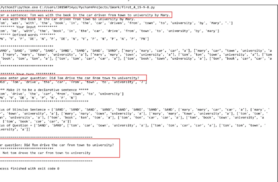
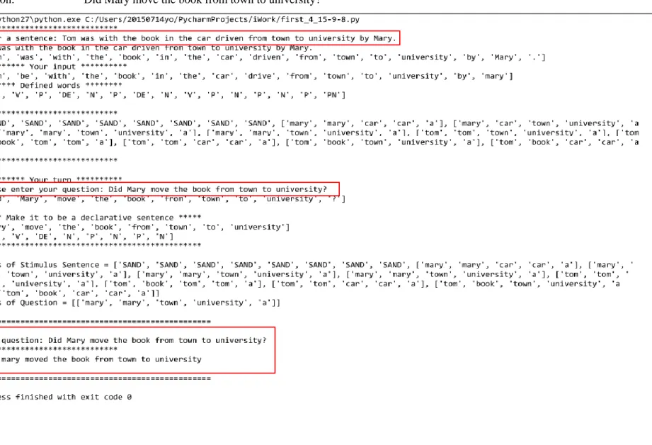
Stimulus sentence: Tom was with the book in the car driven from town to university by Mary. Question: Did Tom drive the car from town to university?