ROW AND COLUMN GENERATION ALGORITHM FOR MINIMUM MARGIN MAXIMIZATION OF RANKING PROBLEMS (Optimization Algorithms : theory, application and implementation)

ROW AND COLUMN GENERATION ALGORITHM FOR MINIMUM MARGIN MAXIMIZATION

OF RANKING PROBLEMS

YOICHIIZUNAGA, KEISUKESATO, KEIJI TATSUMI,AND YOSHITSUGU YAMAMOTO

ABsTliAcT. We consider the ranking problem of learning a ranking function from the data setof objects each of which is endowed withanattribute vector andarankinglabel chosen from the ordered set oflabels. We proposeaprimalformulation with dual representation of normalvector, andthen propose to apply the kerneltechniquetothe formulation. We also propose algorithmsbased ontherowand column generation in order to mitigate the

computational burden duetothelargenumber of objects.

1. INTRODUCTION

This paper is concerned with a multi-class classification problem of $n$ objects, each of

which is endowed with an $m$-dimensional attribute vector $x^{i}=(xi, x_{2}^{i}, \ldots, x_{m}^{i})^{T}\in \mathbb{R}^{m}$ and a label $\ell_{i}$. The underlying statistical model

assumes

that object $i$ receives label $k$, i.e.,

$\ell_{i}=k$, when the latent variable $y_{i}$ determined by

$y_{i}=w^{T}x^{i}+ \epsilon^{i}=\sum_{j=1}^{m}w_{j}x_{j}^{i}+\epsilon^{i}$

falls between two thresholds$p_{k}$ and $p_{k+1}$, where

$\epsilon^{i}$

represents arandom noise whose proba-bilistic property is not known. Namely, attributevectors of objectsare loosely separated by hyperplanes $H(w,p_{k})=\{x\in \mathbb{R}^{m}|w^{T}x=p_{k}\}$ _for $k=1$,2,. . .,$l$ which share a common

normal vector $w$, then each object is given

a

label according to the layer it is located in. Note that neither$y_{i}’ s,$

$w_{j}$’s

nor

$p_{k}$’s

are

observable. Our problemisto find thenormalvector

$w\in \mathbb{R}^{m}$

as

well

as

thethresholds_{$p_{1},p_{2}$}, . . .,$p_{l}$ that best fitthe inputdata$\{(x^{i}, \ell_{i})|i\in N\}.$

This problem is knownasthe rankingproblem andfrequently arises insocial sciencesand operations research. See, for instance Crammer and Singer[2], Herbrich et al. [3], Liu [4], Shashuaand Levin [6] and Chapter8 ofShawe-Taylor and Cristianini[8]. It is a variation of the multi-class classification problem, for which several learning algorithms of the support vectormachine ($SVM$ _forshort) have beenproposed. Werefer the reader to Chapters4.1.2

and 7.1.3 of Bishop [1], Chapter10.10 of Vapnik [10] and Tatsumiet al. [9] and references

therein. What distinguishes the problem from other multi-class classification problems is that the identical normalvector should be shared byallthe separating hyperplanes. In this paper basedon the formulation

_fixed

margin strategy by Shashua and Levin[6],

we

propose

a row and column generation algorithm to maximize the minimum margin for the ranking

problems.

Key words and phrases. ranking problem, Support vector machine, Multi class classification, Kernel

technique, Dualrepresentation.

This paper is organized as follows. We give some definitions and notations in Section 2. In Section3, we formulate the maximization of minimum margin with the hard margin constraints and apply the dual representation of the normal vector to the formulation. In Section4, we propose a

row

and column generation algorithm and prove the validity of the algorithm. In Section5, after reviewing the kernel technique, we apply the kernel technique to the hard margin problem with the dual representation. In Section6, 7 and 8,

weexpand the discussionsso far into the softmargin problem. In Section9, wedemonstrate

an illustrative example for a small instance, then report computational experiments of

our

algorithm in Section 10. In Sectionll, we discuss a desirable property of the separating

curves.

2. DEFINITIONS AND NOTATION

Throughout the paper $N=\{1, 2, . . . , i, . . . , n\}$ denotes the set of $n$ objects and $x^{i}=$

$(Xi, x_{2}^{i}, \ldots, x_{7}^{i_{n}})^{T}\in \mathbb{R}^{m}$ denotes the attribute vector ofobject $i$. The predetermined

set of labels is $L=\{0, 1, . . . , k, . . . , l\}$ and the label assigned to object $i$ is denoted by $\ell_{i}$

.

Let

$N(k)=\{i\in N|\ell_{i}=k\}$ be the set of objects with label $k\in L$, and for notational

conveniencewe write$n(k)=|N(k)|$ for $k\in L$, and $N(k..k’)=N(k)\cup N(k+1)\cup\cdots\cup N(k’)$

for $k,$$k’\in L$ such that $k<k’$. For asuccinct notation we define $X=[$ . . . $x^{i}$ .

. .

$]_{i\in N}\in \mathbb{R}^{m\cross n}$

$X_{W}=[\cdots x^{i}\cdots]_{i\in W}\in \mathbb{R}^{7n\cross|W|}$ (2.1) for $W\subseteq N$, and the corresponding Gram matrices

$K=X^{T}X\in \mathbb{R}^{n\cross n},$

$K_{W}=X_{W}^{T}X_{W}\in \mathbb{R}^{|W|\cross|W|}.$

We denote the $k$-dimensional zero vector andvector of$1$’sby

$0_{k}$ and $1_{k}$, respectively. Given

a subset $W\subseteq N$ and a vector $\alpha=(\alpha_{i})_{i\in W}$ we use the notation $(\alpha_{W}, 0_{N\backslash W})$ to denote the

$n$-dimensional vector $\overline{\alpha}$ such that

$\overline{\alpha}_{i}=\{\begin{array}{ll}\alpha_{i} when i\in W0 otherwise.\end{array}$

3. HARD MARGIN _{PROBLEMS $F$ SEPARABLE CASE}

3.1. Primal Hard Margin Problem. Henceforthwe

assume

that $N(k)\neq\emptyset$ for all $k\in L$

for the sake of simplicity, and adopt the notational convention that $p_{0}=-\infty$ and$p_{l+1}=$

$+\infty$. We say that an instance _{$\{(x^{i}, l_{i})|i\in N\}$} is separable if there exist $w\in \mathbb{R}^{m}$ and

$p=(p_{1},p_{2}, \ldots,p_{l})^{T}\in \mathbb{R}^{l}$ such that

$p\ell_{i}<w^{T}x^{i}<p_{l_{i}+1}$ _for $i\in N.$

Clearly an instance is separable ifand only ifthere are $w$ and$p$ such that

For each $k\in L\backslash \{O\}$

we see

that

$\max w^{T}x^{i}\leq p_{k}-1<p_{k}<p_{k}+1\leq\min w^{T}x^{j},$

$i\in N(k-1) j\in N(k)$

implying

$\min\underline{w^{T_{x^{j}}}}- \max \underline{w^{T}}_{X^{i}}\geq\frac{2}{\Vert w\Vert}.$

$j\in N(k)\Vert w\Vert i\in N(k-1)\Vert w\Vert$

Then the marginbetween$\{x^{i}|i\in N(k-1)\}$ and $\{x^{j}|j\in N(k)\}$_{is at least} $2/\Vert w\Vert$

.

Hence

the maximization of the minimum margin is formulated

as

the quadratic programming

(H) minimize

$\Vert w\Vert^{2}$

subject to $p\ell_{i}+1\leq(x^{i})^{T}w\leq p\ell_{i+1}-1$ for $i\in N,$

or

more

explicitly with the notation introduced in Section 2

(H)

minimize $\Vert w\Vert^{2}$

subject to $1-(x^{i})^{T}w+p_{\ell_{i}}\leq 0$ for _{$i\in N(1..l)$} $1+(x^{i})^{T}w-p_{\ell_{t}+1}\leq 0$ for _{$i\in N(O..l-1)$}

.

Theconstraints therein arecalled hard margin constraints, andwe namethis problem (H)

.

3.2. Dual Representation. A close look at theprimal problem (H) shows that the follow-ing property holds for theoptimum solution $w^{*}$

.

See, for example Chapter 6 of Bishop [1],

Shashua and Levin[6] and Theorem 1 in Sch\"olkopfet al.[7].

Lemma 3.1. Let $(w^{*},p^{*})\in \mathbb{R}^{m+l}$ be an optimum solution

of

(H)

.

Then $w^{*}\in \mathbb{R}^{m}$ lies in

the range space

_of

$X$, i. e., $w^{*}=X\lambda$

for

some $\lambda\in \mathbb{R}^{n}.$

Proof.

Let $w_{1}$ be the orthogonal projection of$w^{*}$ onto the range space of$X$ andlet $w_{2}=$

$w^{*}-w_{1}$. Then

we

obtain

$(x^{i})^{T}w^{*}=(x^{i})^{T}(w_{1}+w_{2})=(x^{i})^{T}w_{1}$ _{for $i\in N,$}

meaning $(w_{1},p^{*})$ is feasible to (H), and

$\Vert w^{*}\Vert^{2}=\Vert w_{1}\Vert^{2}+\Vert w_{2}\Vert^{2}\geq\Vert w_{1}\Vert^{2}.$

Hence by the optimality of$w^{*}$ we conclude that _{$w_{2}=0.$} $\square$

The representation$w=X\lambda$ _is called the dual representation.

Substituting$X\lambda$ for _$w$ yields another primal hard margin problem $(\overline{H})$:

(H) minimize

$\lambda^{T}K\lambda$

subject to $p\ell_{i}+1\leq(k^{i})^{T}\lambda\leq p_{\ell_{i}+1}-1$ for _{$i\in N,$}

where $(k^{i})^{T}=((x^{i})^{T}x^{1}, (x^{i})^{T}x^{2}, \ldots, (x^{i})^{T}x^{n})$ is the ith row of the matrix $K$. Since $n$ is

typically by far larger than $m$, problem (H) might be less interesting than problem (H)

.

Howeverthefact that this formulationonly requiresthe matrix$K$will enablethe application ofkernel technique to the problem.

4. ALGORITHM FOR HARD MARGIN PROBLEMS

In this section, we consider the problem (H) with dual representationof normal vector. The dimension $m$ of the attribute vectors is usually much smaller than the number $n$ of

objects, hence we need a small number of attribute vectors for the dual representation. Furthermore it is likely that most of the constraints areredundant at the optimal solution. We introduce asubset $W$, called working set, of$N$ and consider the following sub-problem.

$(\overline{H}(W))$

minimize $\lambda_{W}^{T}K_{W}\lambda_{W}$

subject to $p\ell_{i}+1\leq(k_{W}^{i})^{T}\lambda_{W}\leq p_{\ell_{i}+1}-1$ for _{$i\in W,$}

where $(k_{W}^{i})^{T}$ is the row vector consisting $(x^{i})^{T}x^{j}$ for _{$j\in W$}

.

We propose to start the

algorithm withasub-problemwhich is much smaller than the problem (H) in both variables and constraints, and increment $W$ as the computation goes on. _{Notethat the dimension of}

$\lambda_{W}$ varies when the size of _$W$ changes as the computation goes on.

Algorithm $RC\overline{H}$ (Row and

Column Generation Algorithm for $(\overline{H})$)

Step 1 : Let $W^{0}$ _be an

initial working set, and let $\nu=0.$

Step 2: Solve $(\overline{H}(W^{\nu}))$ to obtain $\lambda_{W^{\nu}}$ and $p^{\nu}.$

Step 3: Let $\Delta=\{i\in N\backslash W^{\nu}|(\lambda_{W^{\nu}},p^{v})$ violates$p_{\ell_{i}}+1\leq(k_{W^{\nu}}^{i})^{T}\lambda_{W}\leq p_{\ell_{i}+1}-1\}.$ Step 4: If$\Delta=\emptyset$, terminate.

Step 5: Otherwise choose $\Delta^{\nu}\subseteq\Delta$, let $W^{\nu+1}=W^{\nu}\cup\triangle^{\nu}$_{, increment $v$ by 1 and go to} Step 2.

The following lemma shows that Algorithm RCH solves problem (H) upon termination. Lemma 4.1. Let $(\hat{\lambda}_{W},\hat{p})\in \mathbb{R}^{|W|+l}$ be an

optimum solution

_of

$(\overline{H}(W))$.

If

$\hat{p}\ell_{i}+1\leq(k_{W}^{i})^{T}\hat{\lambda}_{W}\leq\hat{p}_{\ell_{i}+1}-1foralli\in N\backslash W$, _(4.1)

then $(\hat{\lambda}_{W}, 0_{N\backslash W})\in \mathbb{R}^{n}$ together with$\hat{p}$

forms

an optimum solution

of

$(\overline{H})$.

Proof.

Note that $((\hat{\lambda}_{W}, 0_{N\backslash W}),\hat{p})$ is a feasible solution of (H) since $(k^{i})^{T}(\begin{array}{l}\hat{\lambda}_{W}0_{N\backslash W}\end{array})=$

$(k_{W}^{i})^{T}\hat{\lambda}_{W},$ $(\hat{\lambda}_{W},\hat{p})$

is feasible to $(\overline{H}(W))$ and satisfies (4.1).

For an optimum solution $(\lambda^{*},p^{*})$ of$(\overline{H})$, let _{$w^{*}=X\lambda^{*},$}

$w_{1}$ be its orthogonal projection

onto the range space of$X_{W}$ and $w_{2}=w^{*}-w_{1}$. Then $w_{1}=X_{W}\mu_{W}^{*}$ for some $\mu_{W}^{*}\in \mathbb{R}^{|W|}$

and

$(\lambda^{*})^{T}K\lambda^{*}=\Vert w^{*}\Vert^{2}\geq\Vert w_{1}\Vert^{2}=(\mu_{W}^{*})^{T}K_{W}\mu_{W}^{*}$ _(4.2)

by the orthogonality between$w_{1}$ and $w_{2}$

.

For $i\in N\cap W$ it holds that

$(k_{W}^{i})^{T}\mu_{W}^{*}=(x^{i})^{T}X_{W}\mu_{W}^{*}=(x^{i})^{T}w_{1}=(x^{i})^{T}(w_{1}+w_{2})$ $=(x^{i})^{T}w^{*}=(x^{i})^{T}X\lambda^{*}=(k^{i})^{T}\lambda^{*},$

which is between $p_{\ell_{i}}^{*}+1$ and $p_{l_{i}+1}^{*}-1$ since $(\lambda^{*},p^{*})$ is feasible to $(\overline{H})$. Then $(\mu_{W}^{*},p^{*})$ is

feasible to $(\overline{H}(W))$. This and the optimality of$\hat{\lambda}_{W}$ yield the

inequality

$(\mu_{W}^{*})^{T}K_{W}\mu_{W}^{*}\geq\hat{\lambda}_{W}^{T}K_{W}\hat{\lambda}_{W}=(\begin{array}{l}\hat{\lambda}_{W}0_{N\backslash W}\end{array})K(\begin{array}{l}\hat{\lambda}_{W}0_{N\backslash W}\end{array})$

.

The two inequalities (4.2) and (4.3) prove the optimality of $((\hat{\lambda}_{W}, 0_{N\backslash W}),\hat{p})$. $\square$

Theorem 4.2. The Algorithm $RCH$ _{solves problem} $(\overline{H})$

.

5. KERNEL TECHNIQUE FOR HARD MARGIN PROBLEMS

The matrix$K$ inthe primal hard margin problem (H) withdual representation of normal vector is composed of the inner products $(x^{i})^{T}x^{j}$ for _{$i,j\in N$}. This enables

us

to apply the

kernel technique simply byreplacing them by$\kappa(x^{i}, x^{j})$ for

some

appropriatekernel function

$\kappa.$

Let $\phi:\mathbb{R}^{m}arrow \mathbb{F}$ be a function, possibly unknown, from $\mathbb{R}^{m}$

to some higher dimensional inner product space $\mathbb{F}$

, so-called the

_feature

space such that $\kappa(x, y)=\langle\phi(x) , \phi(y)\rangle$

holds for $x,$$y\in \mathbb{R}^{m}$, where $\rangle$ is the inner product defined on $\mathbb{F}$

. In the sequel we denote $\tilde{x}=\phi(x)$. The kernel technique considers the vectors $\tilde{x}^{i}\in \mathbb{F}$

instead of$x^{i}\in \mathbb{R}^{m}$, and finds

the normal vector $\tilde{w}\in \mathbb{F}$ and thresholds

$p_{1}$,. . .,$p_{l}$. Therefore the matrices$X$ and$K$ should

be replaced by $\tilde{X}$

composed ofvectors $\tilde{x}^{i}$

and $\tilde{K}=[\langle\tilde{x}^{i}, \tilde{x}^{j}\rangle]_{i,j\in N}$, respectively. Note that

the latter matrix is given

as

$\tilde{K}=[\kappa(x^{i}, x^{j})]_{i,j\in N}$ (5.1)

by the kernel function $\kappa$. The problem to solve is

(H)

minimize $\lambda^{T}\tilde{K}\lambda$

subject to $p\ell_{i}+1\leq(\tilde{k}^{i})^{T}\lambda\leq p_{\ell_{i}+1}-1$ _{for $i\in N.$} Solving $(\tilde{H})$ to find $\lambda^{*}$,

theoptimal normal vector $\tilde{w}^{*}\in \mathbb{F}$wouldbe given

as

$\tilde{w}^{*}=\sum_{i\in N}\lambda_{i}^{*}\tilde{x}^{i},$

which is not available in general due to the absence of an explicit representation of $\tilde{x}^{i\prime}s.$

However, the value of $\langle\tilde{w}^{*},$$\tilde{x}\rangle$ can be computed for a given attribute vector $x\in \mathbb{R}^{n}$ in the

following way:

$\langle\tilde{w}^{*}, \tilde{x}\rangle=\langle\sum_{i\in N}\lambda_{i}^{*}\tilde{x}^{i}, \tilde{x}\rangle=\sum_{i\in N}\lambda_{i}^{*}\langle\tilde{x}^{i}, \tilde{x}\rangle=\sum_{i\in N}\lambda_{i}^{*}\langle\phi(x^{i}) , \phi(x)\rangle=\sum_{i\in N}\lambda_{i}^{*}\kappa(x^{i}, x)$.

Then by locating thethreshold interval determined by$p^{*}$ into which thisvalue falls, we can

assign a label to the new object with $x.$

In the same way as forthe hard margin problem $(\overline{H})$,

we

consider the sub-problem

$(\tilde{H}(W))$

minimize $\lambda_{W}^{T}\tilde{K}_{W}\lambda_{W}$

subject to $p\ell_{i}+1\leq(\tilde{k}_{W}^{i})^{T}\lambda_{W}\leq p_{l_{i}+1}-1$ _{for $i\in W,$} where $\tilde{K}_{W}$ is the sub-matrix consisting of rows and columns of$\tilde{K}$

with indices in $W$, and

$(\tilde{k}_{W}^{i})^{T}$

Algorithm $RC\tilde{H}$ _{(Row and}

Column Generation Algorithm for $(\tilde{H})$)

Step 1 : Let $W^{0}$ be an _{initialworking set,} and let _$v=0.$

Step 2: Solve $(\tilde{H}(W^{v}))$ to obtain $\lambda_{W^{\nu}}$ and $p^{v}.$

Step 3: Let $\Delta=\{i\in N\backslash W^{\nu}|(\lambda_{W^{\nu}},p^{\nu})$ violates $p\ell_{i}+1\leq(\tilde{k}_{W^{\nu}}^{i})^{T}\lambda w\leq p\ell_{i}+1-1\}.$ Step 4: If$\triangle=\emptyset$, terminate.

Step 5: Otherwise choose $\triangle^{\nu}\subseteq\triangle$, let $W^{\nu+1}=W^{\nu}\cup\triangle^{\nu}$, increment $\nu$ by 1 and go to

Step 2.

The validityof thealgorithm is straightforwardfromthe following lemma, whichis proved in exactly the same way as Lemma 4.1

Lemma 5.1. Let $(\hat{\lambda}_{W},\hat{p})\in \mathbb{R}^{|W|+l}$ be an optimum solution

of

$(\tilde{H}(W))$

.

If

$\hat{p}_{\ell_{i}}+1\leq(\tilde{k}_{W}^{i})^{T}\hat{\lambda}_{W}\leq\hat{p}_{l_{i}+1}-1$

for

all$i\in N\backslash W,$

then $(\hat{\lambda}_{W}, 0_{N\backslash W})\in \mathbb{R}^{n}$ together with$\hat{p}$

forms

an optimum solution

of

$(\tilde{H})$.

Theorem 5.2. The Algorithm $RCH$ _{solves problem} $(\tilde{H})$

.

6. SOFT MARGIN PROBLEMS FOR $NoN$-SEPARABLE CASE

6.1. Primal Soft Margin Problems. Similarly to thebinary SVM, introducing

nonnega-tiveslack variables $\xi_{-i}$ and $\xi+i$ for $i\in N$relaxes the hard margin constraints to

soft

margin

constraints:

$p\ell_{i}+1-\xi_{-i}\leq w^{T}x^{i}\leq p\ell_{i+1}-1+\xi+i$ for $i\in N.$

Positive valuesof variables$\xi_{-i}$ and$\xi+i$ meanmisclassification, hencetheyshould beas small as possible. Ifwe penalizepositive $\xi_{-i}$ and $\xi+i$ by adding $\sum_{i\in N}(\xi_{-i}+\xi_{+i})$ to the objective function, we have the following primal

_soft

margin problem with 1-normpenalty.

$(S_{1})$

minimize $\Vert w\Vert^{2}+c1_{n}^{T}(\xi_{-}+\xi_{+})$

subject to $p_{l_{i}}+1-\xi_{-i}\leq(x^{i})^{T}w\leq p_{\ell_{i}+1}-1+\xi+i$ for $i\in N$

$\xi_{-}, \xi_{+}\geq 0_{n},$

where $\xi_{-}=(\xi_{-1}, \ldots, \xi_{-n})$,$\xi_{+}=(\xi_{+1}, \ldots, \xi_{+n})$ and$c$ is apenalty parameter. When 2-norm

penalty is employed, we have

$(S_{2})$

minimize $\Vert w\Vert^{2}+c(\Vert\xi_{-}\Vert^{2}+\Vert\xi_{+}\Vert^{2})$

subject to $p_{\ell_{i}}+1-\xi_{-i}\leq(x^{i})^{T}w\leq p_{\ell_{i}+1}-1+\xi+i$ for $i\in N$

$\xi_{-}, \xi_{+}\geq 0_{n}.$

Lemma 6.1. The nonnegativity constraints on variables $\xi_{-i}$ and $\xi+i$

of

problem $(S_{2})$ are

redundant.

Proof.

Let $(w, \xi_{-}, \xi_{+})$ be a feasible solution of $(S_{2})$ with the nonnegativity constraints

removed. If$\xi_{-i}<0$forsome$i\in N$, replacing it with zerowill reducethe_objectivefunction

value. Therefore $\xi_{-}$ and $\xi_{+}$ are nonnegativeat any optimumsolution of$(S_{2})$.

Thus our problem with 2-normpenalty reduces to

$(S_{2})$

minimize $\Vert w\Vert^{2}+c(\Vert\xi_{-}\Vert^{2}+\Vert\xi_{+}\Vert^{2})$

subject to $p\ell_{i}+1-\xi_{-i}\leq(x^{i})^{T}w\leq p_{\ell_{i}+1}-1+\xi+i$ for $i\in N.$

AsproposedinMangasarian and Musicant [5], theadditionof

a

term $\Vert p\Vert^{2}$tothe objective

function yields the following two formulations $(S_{12})$ and $(S_{22})$

.

$(S_{12})$

minimize $\Vert w\Vert^{2}+c1_{n}^{T}(\xi_{-}+\xi_{+})+d\Vert p\Vert^{2}$

subject to $p\ell_{i}+1-\xi_{-i}\leq(x^{i})^{T}w\leq p_{\ell_{i}+1}-1+\xi+i$ for $i\in N$

$\xi_{-}, \xi_{+}\geq 0_{n},$

and $(S_{22})$

minimize $\Vert w\Vert^{2}+c(\Vert\xi_{-}\Vert^{2}+\Vert\xi_{+}\Vert^{2})+d\Vert p\Vert^{2}$

subject to $p\ell_{i}+1-\xi_{-i}\leq(x^{i})^{T}w\leq p\ell_{i}+1-1+\xi+i$ for $i\in N,$

where $d$ is apenalty parameter.

Naturally,

we

could add to eachofthe above formulations the constraints

$p_{k’}+1-\xi_{-i}\leq(x^{i})^{T}w\leq Pk"-1+\xi+i$ for $k’,$$k”\in L$ _{such that} $k’\leq\ell_{i}<k$

It would, however, inflate the problem size and most of those constraints would be likely redundant. Therefore we willnot discuss this formulation.

6.2. Dual Representation. Obviously we can replace $\Vert w\Vert^{2}$ and $(x^{i})^{T}w$ in each of the primal problems given in the preceding subsection by $\lambda^{T}K\lambda$

and $(k^{i})^{T}\lambda$, respectively, to

obtain theprimal problemwithdualrepresentationof normalvector. Take $(S_{1})$forinstance,

and we have

$(\overline{S}_{1})$

minimize $\lambda^{T}K\lambda+c1_{n}^{T}(\xi_{-}+\xi_{+})$

subject to $p\ell_{i}+1-\xi_{-i}\leq(k^{i})^{T}\lambda\leq p\ell_{i}+1-1+\xi+i$ for$i\in N$

$\xi_{-}, \xi_{+}\geq 0_{n}.$

7. ALGORITHM FOR SOFT MARGIN PROBLEMS

The algorithmforthe softmargin problems may not differsubstantiallyfrom that for the hard margin problems. Take the primal soft margin problem $(\overline{S}_{1})$ with dual representation

of normal vector. The sub-problem to solve is

$(\overline{S}_{1}(W))$

minimize $\lambda_{W}^{T}K_{W}\lambda_{W}+c1_{|W|}^{T}(\xi_{-W}+\xi_{+W})$

subject to $p\ell_{i}+1-\xi_{-i}\leq(k_{W}^{i})^{T}\lambda_{W}\leq p_{\ell_{i}+1}-1+\xi+i$ for $i\in W$

$\xi_{-W}, \xi_{+W}\geq 0_{|W|}.$

We propose the following algorithm for $(\overline{S}_{1})$ in whichwe solve $(\overline{S}_{1}(W))$ repeatedly.

Algorithm $RC\overline{S}_{1}$ (Row and Column Generation Algorithm for $(\overline{S}_{1})$)

Step 2 : Solve $(\overline{S}_{1}(W^{v}))$ to obtain $(\lambda_{W^{\nu}},p^{\nu}, \xi_{-W^{\nu}}, \xi_{+W^{\nu}})$.

Step 3 : Let $\triangle=\{i\in N\backslash W^{\nu}|(\lambda_{W^{\nu}},p^{\nu})$ violates$p\ell_{i}+1\leq(k_{W^{v}}^{i})^{T}\lambda_{W}\leq p_{\ell_{i}+1}-1\}.$ Step 4: If$\triangle=\emptyset$, terminate.

Step 5: Otherwise choose $\Delta^{v}\subseteq\triangle$, let $W^{\nu+1}=W^{\nu}\cup\triangle^{\nu}$, increment $\nu$ by 1 and go to

Step 2.

Lemma 7.1. Let $(\hat{\lambda}_{W},\hat{p},\hat{\xi}_{-W},\hat{\xi}_{+W})$ be an optimum solution

of

$(\overline{S}_{1}(W))$.

If

$\hat{p}\ell_{i}+1\leq(k_{W}^{i})^{T}\hat{\lambda}_{W}\leq\hat{p}\ell_{i}+1-1 foralli\in N\backslash W,$

then $((\hat{\lambda}_{W}, 0_{N\backslash W}),\hat{p}, (\xi_{-W}^{\nu}, 0_{N\backslash W}), (\xi_{+W}^{\nu}, 0_{N\backslash W}))$ is an optimum solution

of

$(\overline{S}_{1})$

.

$f^{)}roof$. First note that $((\hat{\lambda}_{W}, 0_{N\backslash W}),\hat{p}, (\hat{\xi}_{-W}, 0_{N\backslash W}), (\hat{\xi}_{+W}, 0_{N\backslash W}))$ is feasible to $(\overline{S}_{1})$

.

Let

$(\lambda^{*},p^{*}, \xi_{-W}^{*}, \xi_{+W}^{*})$be anoptimumsolution of$(\overline{S}_{1})$, let $w^{*}=X\lambda^{*}$ and

$w_{1}$ be its orthogonal

projection onto the range space of $X_{W}$. Then we

see

that the coefficient vector $\mu_{W}^{*}$ such

that $w_{1}=X_{W}\mu_{W}^{*}$ together with $(p^{*}, \xi_{-W}^{*}, \xi_{+W}^{*})$ forms a feasible solution of $(\overline{S}_{1}(W))$, and

$\Vert w^{*}\Vert\geq\Vert w_{1}\Vert$. Therefore in the same manner as Lemma 4.1, we obtain the desired result.

$\square$

The validity of the algorithm directly follows the above lemma. Theorem 7.2. The Algorithm $RC\overline{S}_{1}$ solves problem $(\overline{S}_{1})$.

8. KERNEL TECHNIQUE FOR SOFT MARGIN PROBLEMS

The kernel technique can apply to the soft margin problem in thesame way as discussed in Section5.

Forthekernel version of soft margin problems with dual representationofnormal vector, we have onlytoreplace $K$by $\tilde{K}$

givenby somekernel function $\kappa$. The kernelversion of$(\overline{S}_{1})$

for instance, is given as

$(\tilde{S}_{1})$

minimize $\lambda^{T}\tilde{K}\lambda+c1_{n}^{T}(\xi_{-}+\xi_{+})$

subject to $p\ell_{i}+1-\xi_{-i}\leq(\tilde{k}^{i})^{T}\lambda\leq p_{\ell_{i}+1}-1+\xi+i$ for _{$i\in N$}

$\xi_{-}, \xi_{+}\geq 0_{n}.$

In the same way as in the previous sectionwe consider the sub-problem of$(\tilde{S}_{1})$, which is

given as

$(\tilde{S}_{1}(W))$

minimize $\lambda_{W}^{T}\tilde{K}_{W}\lambda_{W}+c1_{|W|}^{T}(\xi_{-W}+\xi_{+W})$

subject to $p_{\ell_{i}}+1-\xi_{-i}\leq(\tilde{k}_{W}^{i})^{T}\lambda_{W}\leq p_{\ell_{i}+1}-1+\xi+i$ _{for $i\in W$}

$\xi_{-W}, \xi_{+W}\geq 0_{|W|}.$

Algorithm $RC\tilde{S}_{1}$ (Row and Column Generation Algorithm for $(\tilde{S}_{1})$)

Step 1 : Let $W^{0}$ _be an _{initial working set, and let $v=0.$}

Step 2 : Solve $(\tilde{S}_{1}(W^{\nu}))$ to obtain _{$(\lambda_{W^{v}},p^{\nu}, \xi_{-W^{\nu}}, \xi_{+W^{\nu}})$}.

Step 3: Let $\triangle=\{i\in N\backslash W^{\nu}|(\lambda_{W^{v}}, p^{\nu})$ violates $p\ell_{i}+1\leq(\tilde{k}_{W^{\nu}}^{i})^{T}\lambda_{W}\leq p\ell_{i}+1-1\}.$ Step 4: If$\triangle=\emptyset$, terminate.

Step 5: Otherwise choose $\Delta^{\nu}\subseteq\Delta$, let $W^{\nu+1}=W^{\nu}\cup\triangle^{\nu}$, increment $\nu$ by 1 and go to

Step 2.

We then obtain the following theorem.

Theorem 8.1. The Algorithm $RC\tilde{S}_{1}$ solves problem $(\tilde{S}_{1})$

.

9. ILLUSTRATIVE EXAMPLE

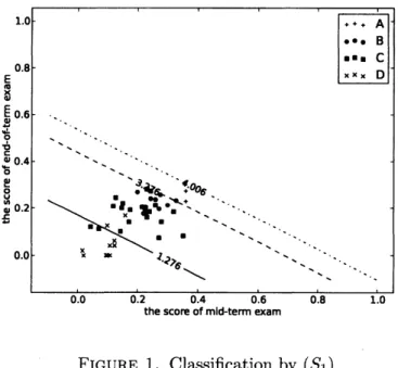
We show withasmall instance howdifferent models result in different classifications. The instance is the grades in calculus of44undergraduates. Each student is given

one

of thefour possible grades $A,$$B,$$C,$ $D$ according to his/her total score of mid-term exam, end-of-term

exam

and

a

number of in-class quizzes. We take the scores of mid-term and end-of-term

exams

to form an attributevector, and the grade

as a

label.

Since the score ofquizzes is not considered

as

an attribute, the instance is not separable.

Hence the hard margin problem (H) is infeasible. The solution of the soft margin problem

$(S_{1})$ with $c=15$ is given in Fig. 1, where students ofdifferent grades are loosely separated

by three straight lines.

FIGURE 1. Classification by $(S_{1})$

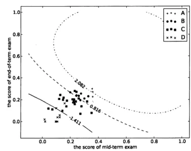
Using the following two kernel functions defined as

$\kappa(x, y)=\exp(-\frac{1}{2\sigma^{2}}\Vert x-y\Vert^{2})$ (Gaussian kernel),

$\kappa(x, y)=(1+x^{T}y)^{d}$ _{(Polynomial kernel)}

with several different values of $\sigma$ and $d$, we solved $(\tilde{S}_{1})$. The result of the Gaussian kernel

with $c=10$ and $\sigma=0.5$ _{is given in Fig. 2, where} one

can

_{observe that the problem} $(\tilde{S}_{1})$

with the Gaussiankernel is exposed to the risk of over-fitting. The result of the polynomial kernel with $c=15$ and $d=4$ is given in Fig.3. From Fig.3, we observe that students of different grades are separatedby three gentle curves.

$FI(_{\grave{J}}URE2$. Classification by $(\tilde{S}_{1})$ with the $Gaussi_{J1}$ kernel

FIGURE 3. Classification by $(\tilde{S}_{1})$ with the polynomial kernel

10. COMPUTATIONAL EXPERIMENTS

We report the computational experimentswith

our

proposedalgorithms. The experiment

was performedon a PC with IntelCore i7, 3.07 GHz processor and 12.0GB of memory. We implemented the algorithms in Python, and used Gurobi5.6.3 as the QPsolver.

We used several randomly generated instances, which are divided into two types. The first type consists of separable instances and the second type consists of non-separable instances. First we generated $n$ attribute vectors $x^{i}=(Xi, x_{2}^{i})$ at random from the unit

square $[0$, 1$]$ $\cross[0$,1$]$

.

Each object $i$

was

assigned alabel

$\ell_{i}\in L=\{0$, 1,.

. .

,3$\}$ according to

the following rule:

$p_{i_{\ell_{\in}}}= \max_{L}\{\ell\in L|_{X}i+x_{2}^{i}>p\ell\}$

where $(p_{0},p_{1},p_{2},p_{3})=(-\infty, 0.5,1.0,1.5)$

.

Then this instance isseparable. Perturbing each

element of the attribute vector, we have

a

perturbed attribute vector $(x_{1}^{i}+\epsilon_{1}^{i}, x_{2}^{i}+\epsilon_{2}^{i})$,

where $\epsilon i$ as well as $\epsilon_{2}^{i}$ is a

random noise following anormal distribution with a zero mean

and

a

standard deviation of 0.03. Then

we

give

a

label $\ell_{i}$ to

an

object $i$ according to the

sumof elements of the perturbed vector instead of the value $xi+x_{2}^{i}$. Due to the presence ofthe randomnoise, the instance is not necessarily separable. We generatefive datasets for each instance with $n$ objects since the results may change owing to the random variables

used in the above instance generation method. We

name

the separable type datasets (the non-separable datasets) “S.n.$q$” (NS.n.q), where $q$ is a dataset ID.

We solved the separable instances by the algorithm$RCH$_{and thenon-separableinstances}

by the algorithm$RC\tilde{S}_{1}$ with _$c=10$

.

In all experiments weused

the polynomial kernel with

a parameter $d=4$. To make the initial working set $W^{0}$, we first calculate the value of

$x_{1}^{i}+x_{2}^{i}$ for each object $i$, and choose three objects whose values

are

the highest, the lowest and the median among objects assigned the

same

label. At Step5 in the algorithms,

we

add at most twoobjects correspondingto the most violated constraints at $(\lambda_{W^{\nu}},p^{\nu})$ to the

current working set $W^{\nu}$ at a time, more precisely, we add the objects $i$ and _{$j\in N\backslash W^{\nu}$}

such that

$i=[argmax]\{1-(\tilde{k}_{W^{\nu}}^{i})^{T}\lambda_{W^{\nu}}+p_{\ell_{i}}^{\nu}>0|i\in N\backslash W^{\nu}\},$

$j=. [argmax]\{1+(\tilde{k}_{W^{\nu}}^{i})^{T}\lambda_{W^{\nu}}-p_{\ell_{i}+1}^{\nu}>0|i\in N\backslash W^{\nu}\}.$

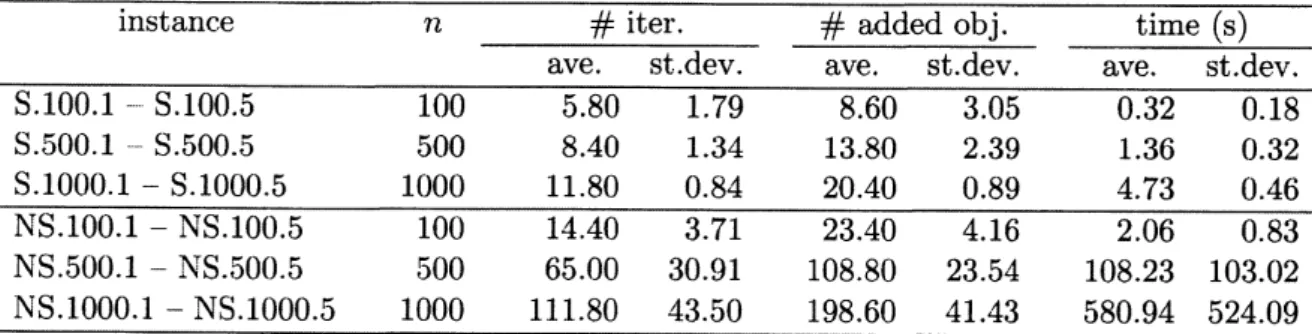
Table 1 shows the results of $RCH$ and $RC\tilde{S}_{1}$ for each instance,

where the columns $\#$

iter , $\#$ added obj.” and

$\langle$

time” represent thenumber ofsub-problems solved,the number of added objects and the computation time in seconds, respectively. The entries “ave.” and “st.dev.” show the average and the standard deviation

across

the five results of

a

corresponding column.

TABLE 1. Results of$RCH$ and $RC\tilde{S}_{1}$

$\overline{\frac{instance.n\frac{\#er}{ave.st.dev}\frac{\#addedobj}{ave.st.dev}\frac{time(s.)}{ave.stdev0.320.18}}{S.100.1-S.l0051005.81.798.603.05}}$

S.500.1 –S.500.5 500 8.40 1.34 13.80 2.39 1.36 0.32

$\frac{S.1000.1-S.1000.5100011.800.8420.400.894.730.46}{NS.100.1-NS.100.510014.403.7123.404.162.060.83}$

$NS.500.1-NS.500.5$ 500 65.00 30.91 108.80 23.54 108.23 103.02

NS.1000.1 –NS.1000.5 1000 111.80 43.50 198.60 41.43 580.94 524.09

From Table 1, weobserve that the number of added objects is much smaller than that of the original problem in the separable case. In the non-separable case, we observe that the number of iterations

as

well as the number of added objects is larger than the separable

11. MONOTONICITY ISSUE

Insomesituations it would be desirable that theseparating

curves

havesome monotonic-ity property, namely an object with attribute vector $x$ be ranked higher than an object with $y$ such that $y\leq x$. Thenwe discuss the monotonicity of the separating curvesin this

section.

Let $P$ be a hyperplane in$\mathbb{F}$

defined by

$P=\{\tilde{x}\in \mathbb{F}|\langle\tilde{w}^{*}, \tilde{x}\rangle=b\}$

for some constant $b\in \mathbb{R}$ and let $C$ denote its inverse image under the unknown function $\phi,$

i. e.,

$C=\{x\in \mathbb{R}^{m}|\phi(x)\in P\}.$

Then $x\in C$ if and only if $\langle\tilde{w}^{*},$$\phi(x)\rangle=b$

.

Since $\tilde{w}^{*}=\sum_{i\in N}\lambda_{i}^{*}\tilde{x}^{i}=\sum_{i\in N}\lambda_{i}^{*}\phi(x^{i})$, we

obtain

$\langle\sum_{i\in N}\lambda_{i}^{*}\phi(x^{i}) , \phi(x)\rangle=b.$

Due to the bi-linearlity of the inner product

we

have

$\langle\sum_{i\in N}\lambda_{i}^{*}\phi(x^{i}) , \phi(x)\rangle=\sum_{i\in N}\lambda_{i}^{*}\langle\phi(x^{i}) , \phi(x)\rangle=\sum_{i\in N}\lambda_{i}^{*}\kappa(x^{i}, x)$,

and then an expression of the inverse image

$C= \{x\in \mathbb{R}^{m}|\sum_{i\in N}\lambda_{i}^{*}\kappa(x^{i}, x)=b\}$

by the kernel function $\kappa.$

Suppose that the kernel function $\kappa(x^{i}, \cdot)$ is nondecreasing for _{$i\in N$}, in the sensethat

$x\leq x’\Rightarrow\kappa(x^{i}, x)\leq\kappa(x^{i}, x$

and $\lambda_{i}^{*}\geq 0$ for $i\in N$

.

Then $\sum_{i\in N}\lambda_{i}^{*}\kappa(x^{i}, x)$ is nondecreasing as awhole.

Lemma 11.1. The kernel

_function

$\kappa(x^{i}, \cdot)$ is nondecreasing and $\lambda_{i}^{*}\geq 0$

for

$i\in N.$ Then

the contours are nondecreasing. The polynomialkernel

$\kappa(x^{i}, x)=(1+(x^{i})^{T}x)^{d}$

is nondecreasing with respect to $x$ if $x^{i}\geq 0$ for $i\in N$. Therefore it would be appropriate to use the polynomial kernel when all the attribute vectors

are

nonnegative including those ofpotential objects, and the monotonicity is desirable. In this case the kernel hard margin problem $(\tilde{H})$ should be added non-negativity constraints of variables $\lambda_{i}’ s$:

(H)

minimize $\lambda^{T}\tilde{K}\lambda$

subject to $p\ell_{i}+1\leq(\tilde{k}^{i})^{T}\lambda\leq p_{\ell_{i}+1}-1$ for _{$i\in N$}

$\lambda\geq 0.$

The problemremains anordinaryconvexquadraticoptimization, and the additional

12. CONCLUSIONS

In this paper, we proposed to apply the dual representation of the normal vector to the formulation based on the fixed margin strategy by Shashua and Levin [6] for the ranking problem. The obtained problemhas the drawback that it has $n$ ofvariables as well as $n$ of

constraints. However the fact that it enables the application of kernel technique outweighs

thedrawback. Then

we

proposed

a row

andcolumn generationalgorithm. Namely,

we

start

the algorithm with

a

sub-problem which is much smaller than the master problem in both variables andconstraints, andincrement both of them

as

the computationgoes on.

Further-more we proved the validity of the algorithm. Through

some

preliminary experiments, our

algorithm performed fairly well. However it should need further research such as a setting of the initial working set $W^{0}$ and achoice of $\triangle^{\nu}$ since aclever choice of these may enhance

the efficiency of the algorithm.

REFERENCES

[1] C.M. Bishop, Pattern Recognition and Machine Learning, Springer, New York, 2006.

[2] K. Crammer andY.Singer, “Prankingwith ranking,” in: T.G.Dietterich,S.Beckerand Z. Ghahramani

eds.,Advances inNeural_informationProcessingSystems 14, MITPress, Cambridge, 2002, pp.641-647.

[3] R. Herbrich, T. Graepeland K. Obermayer, “Large margin rankboundaries for ordinal regression,” in:

A.J. Smola, P. Bartlette, B. Scholkoptand D. Schuurmanseds., Advances in Large Margin Classifiers,

MITPress, Cambridge, 2000, pp.115-132.

[4] T.-Y. Liu, Learning to Rank_{for information}Retrieval,Springer-Verlag, Heidelberg,2011.

[5] O.L. Mangasarian and D.R. Musicant, “Successive overrelaxation for support vector machines,” IEEE Tmnsactions onNeural Networks 10 (1999) 5, 1032-1037.

[6] A. Shashua and A. Levin, “Ranking with large margin principles: two approaches,” in: Advances in

Neural_InformationProcessing Systems 15 (NIPS$2002),2003$,pp.937-944.

[7] B. Sch\"olkopf,R. Herbrich andA.J. Smola, “A generalized representer theorem in: D.Helmbold and B. Williamson eds., Computational Learning Theory, Lecture Notes in ComputerScienceVol. 2111 (2001)

pp. 416-426.

[8] J. Shawe-Taylorand N. Cristianini, Ke veel MethodsforPattern Analysis, CambridgeUniversity Press,

Cambridge, 2004.

[9] K. Tatsumi, K. Hayashida, R. Kawachi and T. Tanino, “Multiobjectivemulticlasssupport vector

ma-chines maximizing geometric margins,” PacificJournal _ofoptimization 6 (2010) 115-140.

[10] V.N. Vapnik, StatisticalLearning Theory, John-Wiley &Sons, NewYork, 1998.

(Y. Izunaga)GRADUATE SCHOOLOFSYSTEMSANDINFORMATIONENGINEERING, UNIVERSITYOFTSUKUBA,

TSUKUBA, IBARAKI 305-8573, JAPAN

$E$-mail address: _{[email protected]}

(K. Sato) SIGNALLING AND TRANSPORT INFORMATION TECHNOLOGY DIVISION, RAILWAY TECHNICAL

RESEARCH INSTITUTE, 2-8-38HIKAR1-CHO, KOKUBUNJI, TOKYO 185-8540, JAPAN

$E$-mailaddress: _{sato. keisuke.}49Qrtri._or.jp

(K. Tatsumi) ELECTRICAL, ELECTRONIC AND INFORMATION ENGINEERING, GRADUATE SCHOOLOF

EN-G1NEER1NG, OSAKA UNIVERSITY, SUITA, OSAKA 565-0871, JAPAN

$E$-mailaddress: tatsumiQeei._eng.osaka-u.ac.jp

(Y. Yamamoto) FACULTY OF ENGINEERING, INFORMATION AND SYSTEMS, UNIVERSITY OF TSUKUBA,

TSUKUBA, IBARAKI 305-8573, JAPAN