ササは本当に強いのか? (新しい生物数学の研究交流プロジェクト)

The

effect of

the

mortality cycle

in two

competitive plants:

Is

Sasa

really advantageous

to

competitior?

ササは本当に強いのか

?

Sungrim

Seirin

Lee (Okayama University) 李聖林*(岡山大学大学院環境学研究科)

Tetsuya Akita(Yokohama National University) 秋田鉄也 (横浜国立大学環境情報学府)

Takashi Kawaguchi (RitsumeikanUniversity) 川口喬 (立命館大学理工学研究科)

Ryo Hironaga (Kyoto University) 広永良 (京都大学生態研究センター)

Abstract 植物は季節や環境変動、簿命などによって様々な死亡サイクルを持つ。例えば、 60年以 上の寿禽を持つといわれるササは、死期が近づくと一斉に開花結実して一斉に枯死する竹の一 種である。ササは、生態系の遷移を著しく遅\langle し、環境を均一化させることで生物の多様性を 大きく下げる。ササが優占になると、被覆により樹木の実生や藁本植物の生育が妨げられる。 このように、ササが競争に非常に強いのは、その一斉死の特徴が原因の一つであると雷われて いる。ササだけではなく、植物の様々な死亡サイクルが生息地や栄養分、光などを巡り競争す る植物の共存に大きな影響を与えるに違いない。ここでは、まず、死亡サイクルが競争する2 つの植物に与える影響を同じ死亡周期をもつ場合とそうでない場合について罐論する。また、 ササ刈りと同時に競争種も一定に減らすことがササの持続的生存を助ける可能性とササの一斉 死が必ずしも競争に有利ではないことを考える。

1

Introduction

In the forest community, theinteractions of plants andcanopy givean effect tothe community structure and dynamics of forest. Plants coexist with competing to dominate over the open spacefor reproduction and seeding, and obtain wateror nutrition. Such acoexistence with the competition is affectedbyenvironmental orhereditary elements such asseasonal variations, life

span and so

on.

The seasonal effect between two competitive plant species has been studied in many lit-eratures ([5], [9], [10]), and has been considered to be important to study the dynamics and

coexistence ofplants. On the other hand, the life span of plants can be considered as the

ele-mentdeterminingthecommunity structure offorest in along-timescale. Thelfespanofplants

hasmuch to do withthe deathrateoftheplants. Thedeathrate ofpopulationisaffectedbythe life span of each individual as well as the enviroIlUlental elements such as seasonal variations.

For example, the dominanceandsimultaneousdeath of Sasa, the dwarfbamboo,h&sagreat

influenceon the regeneration of beech in Japan ([7], [8]). Sasais amonocarpic plantand asort

ofbamboo distributed widely inJapan. It isflowersthen die simultaneously in awide

area

after

rhizomatous vegetative reproduction during a long period. It is reported that the life span of

Sasa is grater than 60 years ([1], [15]). Sasa maintains low death rate for a long time and has

onepeak ofhigh death rate bysimultaneous death,

In this paper, weconsider the effect of the mortality cycle for two competitive plants. Cli-maticchanges orsimultaneouswitheringcanvary the deathratesofplants. Whateffect is given bythemortality cycletocompetitiveplants? Whichmortality$cvclc\backslash$is the mostadvantageousto

competition? Through mathematical analysis and numerical$simulatio\iota ls$, we proposetheanswer about the $q\uparrow\lambda est,i\dot{\iota}$₎$1lS$ above.

Finally, we discuss the effect for humans to mow Sasa. Sasa is usually known as a very

strong plant for competition because other plants almost cannot invade

an

area

where

Sasa

has

already spreadout. People of the past in Japan often

mows

Sasa in order to keep the woods for

livelihood. We show the effect that humans mow Sasa, which can make Sasa be stronger when

it competes against the canopy tree of long periodic death rate or the weeds of short periodic

death rate.

2

Model

The model that

we

consider here is given

as

follows.

$\frac{d}{dt}S=e_{1}S-d_{1}(t)S-a_{1}S^{2}-b_{1}WS$,

$\frac{d}{dt}W=e_{2}W-d_{2}(t)W-a_{2}W^{2}-b_{2}SW$

(1)

where

$d_{1}(t)= \gamma_{1}[\frac{1+\sin(2\pi t/T_{1})}{2}]^{\beta_{1}}$

,

$d_{2}(t)= \gamma_{2}[\frac{1+\sin(2\pi t/T_{2})}{2}]^{\beta_{2}}$

.

Here, $S(t)$ and $W(t)$ denote the densities _{of competing plants.} $e_{i}$ and $a_{i}(i=1,2)$

are

the

reproductive increase rates and intra-specific competition rates of each plant-species. $b_{1}$ and $b_{2}$

are

inter-specific competition rates.

$d_{i}(t)(i=1,2)$

are

the death rates of _the $T_{1}$-periodic

functions of time. $T;(i=1,2)$ are the period of death rate which imply the longevity of

S-species and W-species, respectively. $\gamma_{i}(i=1,2)$ are the maximum values ofdeath rates. The

parameters$\beta_{i}(i=1,2)$ determine thepatternsof distributions ofdeath rates. For_{example, if}$\beta_{1}$

issufficiently large, then the death of the plant $S$ is considered to

occur

simultaneously. Figure 1 shows the graphs _{of the death rate depended}

_on

$\beta_{i}$ with $\gamma_{i}=1$ and $T_{i}=10(i=1,2)$

.

Note

here that all of parameters in the system (1)

are

positive values. Inwhat follows, let

$[d_{i}]= \frac{\gamma_{i}}{T_{i}}\int_{0}^{T_{1}}[\frac{1+\sin(2\pi t/T_{i})}{2}]^{\beta}:dt$

denotes the average of$d_{i}(t)(i=1,2)$

.

3

The effect of the

mortality cycle

in two

competitive

plants

In the system (1),

we

have the solutions $E_{0}=(0,0),$ $E_{S}=(\overline{S}, 0)$, and $E_{W}=(0,\overline{W})$

.

Here $\overline{S}$

is the $T_{1}$-periodic solution ofthe periodic logistic equation;

$\frac{d}{dt}S=(e_{1}-d_{1}(t))S-a_{1}S^{2}$,

provided $e_{1}>[d_{1}]$

,

and $\overline{W}$

is the $T_{2}$-periodic solutionof the periodic logistic equation;

$\frac{d}{dt}W=(e_{2}-d_{2}(t))W-a_{2}W^{2}$

provided $e_{2}>[d_{2}]$ ([3]).

The system (1)has

a

positiveperiodic solution$E_{*}=(S_{*}, W_{*})$ provided$e_{1}>[d_{1}]$ and$e_{2}>[d_{2}]$

([2]). From Theorem 2 and Theorem4 of [4],

we

have the following results.

Proposition 1 $E_{0}$ is stable

if

$e_{1}<[d_{1}]$ and $e_{2}<[d_{2}]$

.

$E_{0}$ is unstable

if

$e_{1}>[d_{1}]$

or

$e_{2}>[d_{2}]$

.

Proposition 2 Supposethat$e_{1}>[d_{1}]$

.

The periodic solution$E_{S}$ islocallyasymptoticallystable

if

and only

_if

$[d_{2}]>e_{2}-[b_{2}\overline{S}]$

.

(2) and is unstable

_if

$[d_{2}]<e_{2}-[b_{2}\overline{S}]$

Proposition 3 Suppose that$e_{2}>[d_{2}]$

.

Theperiodicsolution$E_{W}$ is locally asymptoticallystable

if

and only

_if

$[d_{1}]>e_{1}-[b_{1}\overline{W}]$ (3) andis unstable

_if

$[d_{1}]<e_{1}-[b_{1}\overline{W}]$

.

Proposition 4 Suppose that$e_{1}>[d_{1}]$ and $e_{2}>[d_{2}]$

,

thefolloutng conditions

are

satisfied.

$a_{1}>b_{1}$ and $a_{2}>b_{2}$

.

Then the positive periodic solution$E_{*}$ is locally uniformly stable.

Proposition 4 implies that the two species can coexist if the intra-specific competition ofthe

species is

severer

than the inter-specific competition.W-species (S-species) cannot succeed in

invading ifthe condition (2) (the condition (3)) is

satisfied.

Proposition 2 and Proposition

3

show that the greater the average of death rate of the invasive species is, the moreadvantageous the resident species is. Onthe other hand, the lesser the average of death rate of the invasive species is, the easier theinvasion is.

First,

we

$veri\phi$theeffect ofthe parameter$\beta_{i}$withnumericalsimulations where$T_{1}=T_{2}=30$

.

The parameter vdues of the figures 2, 3,

4

are

given by $e_{1}=3,e_{2}=2,a_{1}=2,a_{2}=1,\gamma_{1}=$

1.5,$\gamma_{2}=1,$$b_{1}=1.5,b_{2}=1$ and

th

$=1$

.

The figures 2, 3,

4

show that S-species cannot invade the habitat of W-species with$\beta_{1}=1$

,

but S-species

can

coexist with W-species when $\beta_{1}$ becomes large. However, if$\beta_{1}$ is sufficiently

large, the two species cannot coexist at the

same

time. S-species always

can

persist but W-species appears only periodically.

Remark 1 In Figure 2, W-species is advantageous to compete againstS-species when$\beta_{1}=\$

.

However, S-species becomes

more

advantageous than W-species when $\beta_{2}$ is large enough. The

death rate

_of

Sasa has the valu$e$

of

$\beta_{i}$ large enough. Thus, a plant

of

small $\beta_{i}$ which has the

same

period utth Sasa is

_difcult

to invade

an

area where Sasa has already spread out. Sasa is advantageous to plants which has the

same

period with

_itself.

Figure2: Thecaseof$\beta_{1}=1$

.

The Figure

3:

The case of _{$\beta_{1}=10$}

.

_{$Fi_{1}re4$}: The case of

$\beta_{1}=300$

.

dotted lineandthesolidline denote The twospecies cancoexist allthe Thetwospeciescancoexist but not

the densities of S-species and W- time. always. W-speciesappearsonlype

species respectively. S-species _{van- riodically.}

ishesastimegoesby.

Inwhatfollows,

we

comsider the

effect

ofthe period ofdeath rates, $T_{i}$ with numerical

simula-tions. We choose the parameter values

as

$e_{1}=3,$ $e_{2}=2,$ $a_{1}=2,$ $a_{2}=1,\gamma_{1}=1.5,\gamma_{2}=1,b_{1}=1$

and $b_{2}=1$

.

We also choose _{$T_{1}=30,$}$\beta_{1}=100$ in $d_{1}(t)$, and $\beta_{2}=1$ in$d_{2}(t)$

.

Let

us

consider the two cases; $T_{2}=10$ and $T_{2}=200$

.

Note herethat

$\frac{1}{mT_{i}}\int_{0}^{mT}:d_{i}(t)dt=\frac{1}{T_{i}}\int_{0}^{T_{i}}d_{1}(t)dt$,

$m$ : natural number.

Thus, we have the

same

average

ofdeath rates$d_{2}(t),$ $[d_{2}]=0.5$, for $T_{2}=10$ and $T_{2}=200$

.

The

average

of death rates $d_{1}(t)$ isgiven by $[d_{1}]=0.085$

.

First, let us consider the _{corresponding averaged system of the system (1) as follows:}

$\frac{d}{dt}S(t)=(e_{1}-[d_{1}])S-a_{1}S^{2}-b_{1}WS$_,

$\frac{d}{dt}W(t)=(e_{2}-[d_{2}])W-a_{2}W^{2}-b_{2}SW$

(4)

Thesystem (4) is the well-known Lotka-Volterrasystem ([13]), and the twospecies

can

coexist, and the equilibrium of the coexistence is globally asymptotically stable when $a_{2}(e_{1}-[d_{1}])$ –

$b_{1}(e_{2}-[d_{2}])>0$ and $a_{1}(e_{2}-[d_{2}])-b_{2}(e_{1}-[d_{1}])>0$

.

This condition holds when $a_{1}>b_{1}$ and

$a_{2}>b_{2}$

,

that is, the intra-specific competition is stronger than the inter-specific competition.

Now, _{the numericalsimulation results}

_are

_{given by the following figures 5,6,7.}

$*=$ $S(t)$ $\vee-\aleph’$

.

名.

..

$W(t)$

.

$-$ $-$ $-$ $\sim_{ti}$渦 $-$ $-$ $-$

Figure 5: The case of average Figure6: Thecaseoftheperiodic Figure 7: Thecaseof theperiodic

deathratesystem. The two species system (1). $T_{1}=30,$$\beta_{1}=100,T_{2}=$ $8y_{8}tem(1)$

.

$T_{1}=30,$ $\beta_{1}=10,T_{2}=$ coexist, but W-species maintains 10 and $\beta_{2}=1$

.

Two species can 200and $\beta_{2}=1$

.

W-species has the

verysmall density astime goes to. coexist. period that it goes toextinction.

InFigure 5, the twospecies coexist, _{but W-species almost dies out and remains only slightly}

as

time

goes

to infinity when

we

choosethe deathrate

as

the averageofit. InFigure 6, however, the periodic death rate makes _{W-species coexist with S-species and have greater density than}

that of Figure 5. We give the greater period $T_{2}$ of W-species in Figure 7 than that ofFigure 6.

Then, Figure 7 shows that two specie

can

coexist but not always. W-species hasa period where it goes to extinct.

Remark 2 When the two species have the

same

periods

_of

death rates, the smaller$\beta_{i}$ is

advan-tageous to compete because the average

_of

death rate becomes smaller (Figure 1 and Figure 2). However, Figure 6 shows thatW-species can have the higher density than that

_of

the

case

_of

the average death rate when it has a properperiod $T_{2}$ (here $T_{2}=30$) when$\beta_{2}$ is greater than$\beta_{1}$

.

If

$T_{2}$ is large enough, then W-species is

more

disadvantageous to competition than that

of

the

case

of

$T_{2}=30$ because it has $a$ extinct period. Even though W-species has the

same

average death

rate in Figure

6

and Figure 7, the longerperiod gives the disadvantage

_for

competition. Remark 3 For the averaged system (4),

we

have the followingproperties $(/13J)$:

(i) Either the equilibrium $(0, (e_{2}-[d_{2}])/a_{2})$

or

the equilibrium $((e_{1}-[d_{1}])/a_{1},0)$ is globally

asymptotically stable

_if

$\{a_{2}(e_{1}-[d_{1}])-b_{1}(e_{2}-[d_{2}])\}\{a_{1}(e_{2}-[d_{2}])-b_{2}(e_{1}-[d_{1}])\}<0$

,

(ii) A positiveinterior equilibrium enists

_if

$\{a_{2}(e_{1}-[d_{1}])-b_{1}(e_{2}-[d_{2}])\}\{a_{1}(e_{2}-[d_{2}])-b_{2}(e_{1}-$ $[d_{1}])\}>0$

,

andit is unstable

if

$a_{2}(e_{1}-[d_{1}])-b_{1}(e_{2}-[d_{2}])<0$ and$a_{1}(e_{2}-[d_{2}])-b_{2}(e_{1}-[d_{1}])<0$

.

However,

we

should notice that

a

nontrevialpositiveperiodic solution

can

exist in the system

(1)

even

_if

$\{a_{2}(e_{1}-[d_{1}])-b_{1}(e_{2}-[d_{2}])\}\{a_{1}(e_{2}-[d_{2}])-b_{2}(e_{1}-[d_{1}])\}<0$ is

satisfied.

Moreover, $a$

nontrivialpositive periodic solution

can

exist in the case

_of

either$a_{2}(e_{1}-[d_{1}])-b_{1}(e_{2}-[d_{2}])<0$

or

$a_{1}(e_{2}-[d_{2}])-b_{2}(e_{1}-[d_{1}])<0([12J)$

.

That is, the periodic death rate may

cause

the two species to coexist

even

_if

the comsponding averaged system wotdd

_force

either

_of

the two species

to extinction.

4

Sasa is

really advantageous

to

competitor ?

Sasa flowers then die simultaneously after rhizomatous vegetative reproduction during greater

than

60

years. It is reported that understory bamboo abundance influence long-term stand structure and development ofcanopytree by suppressing three recruitment ([14]). Thus Sasa is

usually considered to bevery strong to compete.

The dynamicsofSasahave been studiedin many papers ([6], [7], [8], [11], [14]), especially

as

a

lattice-structured model ([6]) and

an

individual based model ([7]). In Japan, Sasa produces a

inhibiting effect

on

the regeneration ofbeech and hasa veryharmful effect

on

the sustainability of beech stand, which depends

on

the longevity of Sasa ([6], [8]). In this section, we discuss

thedynamicsofSasa with

a

deterministicmodel ofordinarydifferential equationsby numerical simulations.

First,letusnote that $[d_{i}]$is

a

non-increasingfunctionfor$\beta_{i}$because$(1/2)+(1/2)\sin(2\pi t/T_{1})\leqq$

1. Thus, $[d_{i}]$ becomes small when$\beta_{i}$becomes large. InSection3,

we

also haveknown that

stabil-ity results depend on the average deathrates of the two species. A plant which dies simultane-ously such

as

Sasa has

a

sufficiently large $\beta_{i}$

,

andthus

we

can

considerSasa to be advantageous

to compete. However,

we

showthatthe simultaneous death ofSasa is not decisive

cause

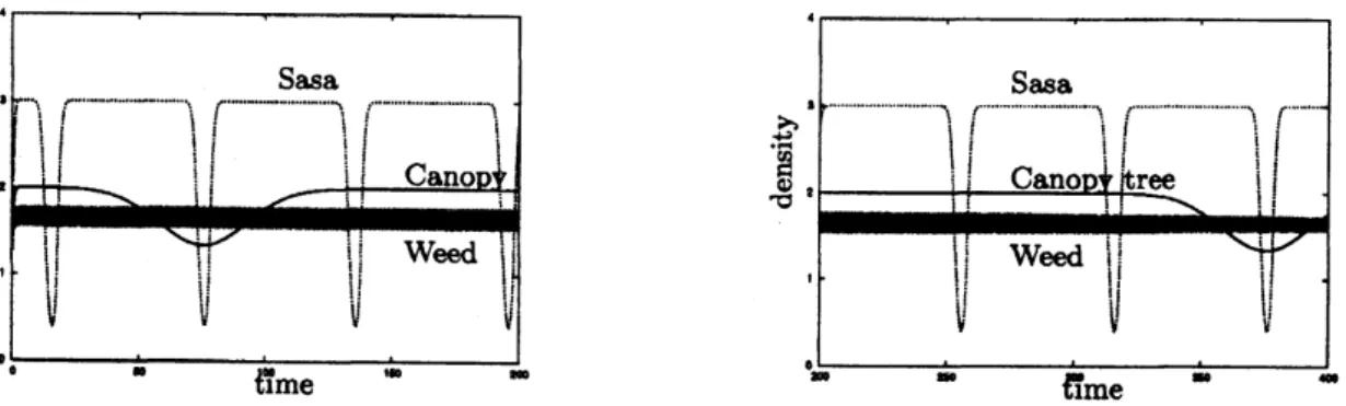
for the advantage ofSasabynumerical simulations.

In what follows, $S(t)$ denotes the densityof

Sasa

inthesystem (1). Notethat Sasa maintains low death rate for

a

longtime and has

one

peak of high death rate by simultaneous death. Let

us

choose

a

properthe parameter values which implies the life pattern ofSasa

as

follows:

$e_{1}=3$, $\gamma_{1}=3$

,

$a_{1}=1$

,

$\beta_{1}=50$

.

(5)

Here,

we

set the life span of

Sasa

at

60

years, that is, $T_{1}=60$

.

We alsoconsider the two kinds of competitive plants agaimst Sasa; A canopy three of a long longevity and

a

weed of

a

short

a similar time can have a high death rate in the end of the time of longevity. Thus, we set

$T_{2}=300$ years and $\beta_{2}=15$ in the case of canopy tree. In the case of

some

weeds of short

longevity, we choose $T_{2}=1$ year and $\beta_{1}=1$. The other parameter values

are

given by

$e_{2}=3$, $\gamma_{2}=1$, _{$a_{2}=1.5$}, $b_{1}$(canopy) $=1.44$

,

$b_{1}$(weed) $=1.67$, $b_{2}=0.5$

.

(6)

The time variationsof thedensitiesof the three species without acompetitor aregiven byFigure 8.

Figure

8:

Dynamics of Sasa, Canopythreeand Weed withoutacompetitor. The left and right figures describe

the density’svariation of eachspecies from$0$year to200yearsand from200yearsto400years, respectively. The

weeds have very smallperturbations.

Now,

we

consider the effect that humans

mow

Sasa

as

well as the competitive plants of it. We suppose that the mowing by humanI is done constantly, and thus the decreasing rates by

mowing of Sasa and the competitive plant

are

given by constants. The model discussed here is

as follows:

$\frac{d}{dt}S(t)=(e_{1}-d_{1}(t)-a_{1}S-b_{1}W)S-c_{1}S$,

$\frac{d}{dt}W(t)=(e_{2}-d_{2}(t)-a_{2}W-b_{2}S)W-c_{2}W$_,

(7)

where $q(i=1,2)$

are

the decreasing rates for humans to

mow

Sasa

and W-species.

Let

us

choose the values of $c_{1}$ and $c_{2}$ as

0.7

and 1.2, respectively. Then, the simulation

results, Figure 9 and Figure 10, show that Sasa

can

still exist if humans

mow

the competitors

as

well as _{Sasa, and it is advantageous to the competitors because the densities’ variations of} thecompetitors

are

determined by the period of Sasa.

Figure

9:

The case that Sasa competes to Figure

10:

The case that Sasa competes to

Now, let

us

remove

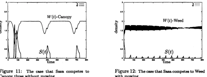
the effect by mowing in the system (7). We choose the same parameter values above, (5) and (6). And we choose $c_{i}=0(i=1,2)$. Then the numerical results are given

by the figures 11, 12.

Figure 11: The case that Sasa competes to Figure 12: Thecasethat Sasa competestoWeed

Canopy threewithoutmowing. with mowing.

Figure 11 and Figure

12

show that

Sasa

is disadvantageous to the two competitor,

canopy

three and weed. As

a

results, the effect that humans

mow

Sasa

can

make Sasa to be stronger tocompete against the canopy three oflong periodic deathrate and the weed ofshort periodic death rate.

Remark 4 The average death rates

_of

Sasa, canopy threeandweed

are

given by$[d_{sasa}]=0.239$

,

$[d_{\infty n\varphi y}]=$

0.145

and $[d_{weed}]=0.5$

,

respectivdy. When Sasa competes urith canopy three, the

property (i)

_of

Remark

3

is

_{satisfied for}

the parameter values chosen in Figure 11. In the

case

thatSasa competes with weed, theproperty (ii)

_of

Remark3is

_satisfied

_for

the parameter values chosen in Figure 12. The simulation results

_of

Figure 11 and Figure 12 show that a nontrivial

positiveperiodic solutionexists in the system(1)

even

_if

thecorresponding averaged systemwould

fonce

either

_of

the two species to extinction.

References

[1] J. J. N. Campbell, Bamboo floweringpattem: A global viewwith special

_reference

to East

Asia, J. Am. Bamboo Soc., 6 (1985)

17-35.

[2] J. M. Cushing, Stable limit cydes

_of

time dependent multispecies interactions, Math.

Bioscience, 31 (1976)

259-273.

[3] J. M. Cushing, Stable positive periodic solutions

_of

the time-dependent logistic equation underpossible hereditary influences, J. Anal. Appl., 60 No. 3 (1977)

747-754.

[4] J. M. Cushing, Two species competition in a periodic environment, J. Math. Bio., 10 (1980)

385-400.

[5]

J.

M. Cushing, Periodic

Lotka-Voltem

competition equations,

J. Math.

Bio., 24 (1986)

381-403.

[6] K. Kawano and Y. Iwasa, A

lattice-structured

modd

_for

beech

_forest

dynamics: the

_effect

of

understory

_dwarf

bamboo

,

Ecological Modeling, 66 (1993)

261-275.

[7] T. Kubo and H. Ida, Sustainability

_of

an

isolated

_beech-dwarf

bamboo stand: analysis.

_of

forest

dynamics utth individual based model, Ecological Modeling, 111 (1998)

223-235.

[8] T. Nakashizuka, Regeneration

_of

Beech (fagus crenata)

_after

the simultaneous death

_of

undergroutng

_dwarf

bamboo (Sasa kurilensis) Ecol. $R\epsilon s,$ $3$ (1988)

21-35.

[9] T. Namba, Competitive co-existence in aseasonallyfluctuating $en\dot{w}ronment$ J.theor.Biol,

111 (1984)

369-386.

[10] T. Nambdaand

S.

Takahashi, Competitive coesistence in

a

seasonally fluctuating

environ-ment II. Multiple stable states and invasion suocess, Theoretical Population Biology, 44

(1993)

374-402.

[11] A. Makita, Y. Konno, N. Fujita, K. Takada and E. Hmabata, Recovery

_of

a

Sasa tsuboiana population

_after

mass

_flowerin9

and death Ecol. Research, 8 (1993)

215-224.

[12] P. de MottoniandA. Schiaffino, Competition system withpenodic

_{coefficients:}

Ageometric approach J. Math. Bio, 11 (1981)

319-335.

[13] N. Shigesada and K. Kawasaki, “Biological Invasions: Theory and Practice,”Oxford

uni-versity press,

1997.

[14] _{A. H. Taylor, H. Jinyan and Z. ShiQiang, Canopy three development and$unde y vwth$}

bam-boo dynamics in old-grvwth

Abies-Betula

_forests

in southwestem China: $a$ 12-yearstudy,

Forest Ecology and Management,

200

(2004)

347-360.

[15] K. Ueda, On theflowenng and deaath

_of

bamboos and the$p$roper treatment. (II) Relation

between the

_flo

wing

bamboo

and a rhizome system in the bamboo gevve utth

non

flowering