Approximations of reaction-diffusion equations by interface equations : boundary-interior layer (Conference on Dynamics of Patterns in Reaction-Diffusion Systems and the Related Topics)

(1)

Approximations of

_{reaction-diffusion}

_equations

by

interface

equations

-boundary-interior layer

-広島大学・理学研究科坂元国望 (Kunimochi SAKAMOTOJ)

Department ofMathematical and LifeSciences,

Graduate

SchoolofScience, Hiroshima University

1 Introduction.

We_{deal with transition layers of the}_following _scalar_{reaction-diffusion} _equation

(1.1) $\{$

$u_{t}= \Delta u+\frac{1}{\epsilon^{2}}f(u)$ (in $\Omega$, $t>0$) $\frac{\partial u}{\partial \mathrm{n}}=0$ (on $\partial\Omega$, $t>0$)

with the homogeneous Neumann _{boundary conditions. This system, called the}

Allen-Cahn

equation, has been studied extensively for

bistable

reaction kinetics.

Atypical example of the nonlinearity $f$ is acubic polynomial $f(u)=u-u^{3}$

.

In

general,

we assume

that the nonlinearity $f$ is obtained from

adouble-well

potential

$F(u)$ of equal depth. Namely, _$f(u)=$

_-Ff{u)

_with _{$F(u)\geq 0$} _{attains its}

_absolute

minimum atexactlytwo non-degenerate critical points$u=\pm 1$ (on-degereracy _here

means

that $F’(\pm 1)>0)$

.

_{These conditions}

_ensure

_the_existence_{of aspecial}_solution

$Q(z)(z\in \mathrm{R})$, called astanding

wave

solution, which satisfies

(S-W) $\frac{d^{2}Q}{dz^{2}}+f(Q)=0$, _$z$ $\in \mathrm{R}$,

$\lim_{zarrow\pm\infty}Q(z)=\pm 1$, $Q(0)=0$

.

The function $Q(z)$ will play important roles in this paper.

The domain 0is asmooth, bounded

one

in $\mathrm{R}^{N}$

,

$\mathrm{n}$ stands for the unit inward

normalvector

on

$\partial\Omega$, and the parameter

$\epsilon$ $>0$ is small.

Our main

concern

in this paper is to show the existence of internal transition

layers which exhibit asharp transition ffom $u\approx-1$ to $u\approx+1$

across

such $\mathrm{a}$

hypersurface $\Gamma$ that intersects the boundary

of the domain; $\overline{\Gamma}\cap\partial\Omega$

$\neq\emptyset$

.

We call

this _{kind of internal transition} _layer _{aboundary-interior}_layer.

_We

_also _analyze_the

stability property of boundary-interior _{layers by using}

_some

_geometric

_information

of$\Gamma$,$\partial\Omega$ and$\partial\Gamma\subset\partial\Omega$

.

When $\epsilon>0$ is small, the solutions of (1.1) for aclass of

initial

functions

are

known to_{develop transition layers within}_{ashort time scale} _of$O(\epsilon^{2}|\log\epsilon|)[3]$

.

This

phenomenon is caused by the_{strong bistability of the ordinary differential} _equation

数理解析研究所講究録 1330 巻 2003 年 134-148

(2)

$u_{t}=\tau_{\epsilon}^{1}f(u)$ with $u=\pm 1$ being stable equilibria. According to the sign of the

value of the initial function, the solution is quickly attracted to either $u=+1$ or

$u=-1$, thus creating asharp transition from $u\approx-1$ to $u\approx 1$

near

the set, called

an

interface,

$\Gamma(t):=\{x\in\Omega|u^{\epsilon}(u, t)=0\}$

.

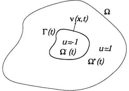
The interface divides $\Omega$ into two sub-domains $\Omega^{\pm}(t)$ (cf. Figure 1) defined by

$\Omega^{\pm}(t):=\{x \in\Omega|\pm u^{\epsilon}(x, t)>0\}$

.

When $x\in\Omega^{\pm}(t)$, $u^{\epsilon}(x, t)arrow\pm 1$

as

$\mathit{6}arrow 0$

.

Such solutions with sharp transition

are

called transition layersolutions.

Figure 1: The$\mathrm{i}$ terface

$\mathrm{T}(\mathrm{t})$ andthe normal vector $\nu(x, t)$

.

Itisalsowell known (cf. [3],forinstance)thatthe interface$\Gamma(t)$evolvesaccording

to its

mean

curvature:

(1.2) $\mathrm{V}_{\Gamma(t)}(x)=-\kappa(x;\Gamma(t))(x\in\Gamma(t), t>0)$

where $\mathrm{V}_{\Gamma(t)}(x)$ is the speed of the interface measured along the unit normal $\nu(x, t)$

of$\Gamma(t)$ at$x$ ($\nu$pointstothe $\Omega^{+}(t)$-side,cf. Figure 1) and $\kappa(x;\Gamma)$ stands for the

sum

of the principal curvatures of $\Gamma$ at _$x\in\Gamma$. Hereafter, $\kappa$ is simply called the

mean

curvature and the equation (1.2) is referred to

as

the

mean

curvature flow. To be

precise about the sign of$\kappa$ (which is theopposite to geometers’ convention), let

us

extend theunit normal vector$\nu$to aneighbourhoodof$\Gamma$

.

Then

our mean

curvature

is defined

as

the divergence of$\nu$;

$\kappa(x;\Gamma)=\mathrm{d}\mathrm{i}\mathrm{v}\nu(x)$, $x\in\Gamma$.

(3)

When the interface$\Gamma(t)$ staysawayfrom the boundary$\partial\Omega$, the dynamics of (1.2)

has been studied rather extensively ([6, 8]). In such acase, the interface governed

by the

mean

curvature flow (1.2) does not feel the presence of the boundary

an.

Therefore, the domain $\Omega$ does not play anyrole in the dynamics of (1.2).

Our

concern

inthispaper,

on

theother hand, is the

case

where theinterface$\Gamma(t)$

intersects the boundary $\partial\Omega$ (cf. Figure2). The motion of

$\Gamma(t)$ in such asituation is

still described by the

mean

curvature flow (1.2) to the lowest orderapproximation.

Main questions

we

raisein this article

are:

When (1.2) has an equilibrium interface, does it give rise to

an

equilib-riumboundary-interiorlayer for $($1.1$)^{}$ If the

answer

is affirmative, what

is it that determinesthe stability of the layer?

Thedynamicsof such interfaces intersecting the boundary of domain has been

stud-ied by several authors ([2, 13, 4, 5, 12, 15, 10]).

Since

we

have identified $\Gamma(t)$

as

the 0-level set ofthe solution to (1.1), the ho

mogeneous

Neumann boundary conditions demand that $\Gamma(t)$ be perpendicular to

$\partial\Omega$ at theintersection $\partial\Gamma(t)=\overline{\Gamma(t)}\cap\partial\Omega$

.

Therefore, the interface

$\Gamma(t)$ immediately

feelsthe presence ofthe boundary, and the geometryof

an

influences

thedynamics

of(1.2).

Figure 2: The interface intersecting the boundary.

Theexistenceof energy-minimising solutions (of (1.1)) with interfaceintersecting

the boundary

was

first rigorously established in [15] by avariational method. For

competition-diffusion systems, stable internal layers intersecting the boundary

was

established in [12] for rotationallysymmetric domains. Exponentially slow motions

offlat interfaces arediscussed in $[2, 13]$, where interfaces intersect flat parallel part

of the boundary. Motions of interfaces with contact angle

was

treated in [4] for

a

generalized

mean

curvature

flow.

Dynamics offlat interfaces in astrip like domain

was

discussed in [5], wherethespeed of the interface is of order$O(\epsilon^{2})$ withrespectto

(4)

thetime scale of(1.1). In [10], the existence and stability ofequilibrium

boundary-interior layers with flat interfaces were established. Recently, the

same

results

as

[10] have been obtained by [14] via different methods. In all of these works, the

geometryofthe boundary

an

has essential effects

on

the dynamics of (1.1).

The purpose of this article is to extend the results in [10] and [14] to

higher-dimensional domains.

2Review

of

tw0-dimensional results.

In thissection we

assume

$N=2$, _{and review know} results according to [10].

In order to describe

an

equilibrium interface$\Gamma$ of (1.2), let

us

consider the

dis-tance

function

$L$;

L:an x

$\partial\Omegaarrow[0,\infty)$, $L(p,q)=\mathrm{d}\mathrm{i}\mathrm{s}\mathrm{t}(p,q)$

.

Theorem2.1 (Equilibrium Interface).

_If

$(p_{\mathrm{r}}, q_{*})\in\partial\Omega$

x

an

satisfies

following

conditions:

(i) $(p_{\mathrm{r}}, q_{\mathrm{r}})$ is

a

critical point

of

$L$;

(ii) $L_{*}:=L(p_{*}, q_{*})>0$;

(iii) the open straight line-segment$\overline{p_{*}q_{*}}is$ contained in $\Omega$,

then, $\Gamma=\overline{p_{*}q_{*}}is$

an

equilibrium

interface

of

(1.2).

Conversely,

any

equilibrium

_of

(1.2) is characterized by theseproperties.

Proof.

In the two dimensionalcase, $\kappa=0$ is equivalentto $\Gamma$being astraight line. It

isverifiedthat $\partial L(p_{*}, q_{*})/\partial p=0$is equivalentto$\overline{p_{*}q_{*}}1_{\mathrm{P}*}\partial\Omega$

.

Also, $\partial L(p_{*}, q_{*})/\partial q=$

$0$ isequivalent to $\overline{p_{*}q_{*}}[perp]_{q}$

.

$\partial\Omega$. Now, the statementsofthe theorem follow. $\square$

We

now

define thecurvature of$\partial\Omega$ with respect to its inwardunit normal $\mathrm{n}$ by

$\overline{\kappa}_{\mathrm{p}}=\mathrm{d}\mathrm{i}\mathrm{v}\mathrm{n}(p)$, $p\in\partial\Omega$.

Let

us

denote by $\overline{\kappa}_{p}$

.

and $\overline{\kappa}_{q_{*}}$ the cruvature of

an

at the two end points of the

equilibrium interface $\Gamma=\overline{p_{*}q_{*}}$

.

Let

us

define $\mathrm{D}$ and$\mathrm{T}$ by

$\mathrm{D}:=\overline{\kappa}_{\mathrm{p}}$

.

$+\overline{\kappa}_{q}$

.

$+L_{*}\overline{\kappa}_{p_{*}}\overline{\kappa}_{q}.$,

$\mathrm{T}:=2+L_{*}(\overline{\kappa}_{p_{\mathrm{r}}}+\overline{\kappa}_{q}.)$

.

These quantities

are

related to the second variation of$L$

.

Namely, $\mathrm{T}/L_{*}$ and $\mathrm{D}/L_{*}$

are, respectively, the trace and determinant of the Hessian matrix (i.e., the second

variation) of$L$ at $(p, q)=(p_{\mathrm{r}}, q_{*})$

.

(5)

Theorem 2.2 (Existence of boundary-interior layers).

Assume

that the

fol-lowing non-degeneracy condition is

_satisfied

(a) $\mathrm{D}\neq 0$

.

Then there eist

an

$\epsilon_{*}>0$ and afamily

of

equilibrium solutions $U^{\epsilon}(x)$

of

(1.1)

for

$\epsilon$ $\in(0, \epsilon_{*}]$, enjoying thefollowing properties:

(i) For each$\delta$ $>0$,

$\lim_{\epsilonarrow 0}U^{\epsilon}(x)=\{$ $-11$ uniformly in $\{$$x\in \mathrm{d}\overline{\frac{\Omega}{\Omega}}-,\mathrm{i}\mathrm{s}\mathrm{t}(x,\Gamma)>\delta x\in \mathrm{d}\mathrm{i}\mathrm{s}\mathrm{t}(x,\Gamma)>\delta+,$

.

(ii) Near the

_interface

$\Gamma$, the solution

$U^{\epsilon}(x)$ has the asymptotic characterization:

$U^{\epsilon}(x) \approx Q(\frac{\mathrm{d}\mathrm{i}\mathrm{s}\mathrm{t}(x,\Gamma)}{\mathit{6}})$ ,

where $Q(z)(z\in \mathrm{R})$ is the standing

wave

solution in (S-W).

Let

us

call such asolution

as

in Theorem 2.2 aboundary-interior layer. The

stability properties of the boundary-interior layeris given in the followingtheorem.

In Theorem 2.3 below, the Morse index of

an

equilibrium solution to (1.1)

means

the number ofunstable (positive) eigenvaluesfor the eigenvalue problem

(2.1) $\lambda\phi=\Delta\phi+\frac{1}{\epsilon^{2}}f’(U^{\epsilon})\phi$ in $\Omega$, $\frac{\partial\phi}{\partial \mathrm{n}}=0$

on

an,

associated with the linearized operator around the equilibrium $U^{\epsilon}$ of (1.1). Also, in

the

same

theorem, the Morse index ofacritical point $(p_{*}, q_{*})$ of $L$ is the number of

positive eigenvalues of the Hessianmatrix $\mathrm{o}\mathrm{f}-L$ at _{$(p, q)=(p_{l}, q_{*})$}

.

Theorem 2.3 (Stability property ofboundary-interior layers). Let $U^{\epsilon}(x)$ be

the solution in Theorem 2.2. As

an

equilibrium solution

_of

(1.1), it is

(1) stable (the Morse index 0), if$\mathrm{D}>0$ and$\mathrm{T}>0$,

(2) unstable,

_if

otherwise, with

(2-i) the Morse index

_1if

$\mathrm{D}<0$

(2-ii) the Morse

inde

$ex2$

if

$\mathrm{D}>0$ and$\mathrm{T}<0$

.

(3) The Morse index

_of

the equilibriumsolution describedin items (1) and(2)

are

the

same as

the Morse index

_of

the corresponding critical point $(p_{*}, q_{*})$

for

the

$fi\iota nction$ $L(p, q)$

.

(6)

Theorems 2.2 and 2.3 says that the dynamics of boundary-interior layers are

qualitatively described by the gradient system of the function $L$. It is easy to

see

that Theorems 2.2 and 2.3

are

restatements ofTheorems 1.3 and 1.4 in [10].

Inorder to gain

some

insightsfor Theorem 2.3, it is illuminating to consider the

following eigenvalue problem

(2.2) $\{$

$\phi_{\tau\tau}(\tau)=\lambda\phi(\tau)$, $\tau\in(-\frac{L}{2}., \frac{L}{2}.)$,

$\phi_{\tau}(-\frac{L}{2}.)-\overline{\kappa}_{q}.\phi(-\frac{L*}{2})=0$

$- \phi_{\tau}(\frac{L}{2}.)-\overline{\kappa}_{p*}\phi(\frac{L_{\mathrm{s}}}{2})=0$

.

This is

an

eigenvalue problemassociated with the linearizationof(1.2)

on

the

equi-libriuminterface$\Gamma=\overline{p_{*}q_{*}}$

.

It

was

shownin [10] that non-criticaleigenvaluesof(2.1)

go$\mathrm{t}\mathrm{o}-\infty$

as

$\mathit{6}arrow 0$andthat critical eigenvalues of(2.1)

converge

to the eigenvalues

of(2.2). It is rather elementary to show that (2.2) has

1.

no

positive eigenvalues andno 0-eigenvalue if$\mathrm{D}>0$ and $\mathrm{T}>0$;

2.

one

positive eigenvalue and

no

0-eigenvalue if$\mathrm{D}<0$;

3. two positive eigenvalues and no 0-eigenvalue if$\mathrm{D}>0$ and $\mathrm{T}<0$;

4.

one

0-eigenvalue and

no

positive eigenvalue if$\mathrm{D}=0$ and $\mathrm{T}>0$;

5.

one

0-eigenvalue and

one

positive eigenvalue if$\mathrm{D}=0$ and $\mathrm{T}<0$

.

Note that it is impossible to have both $\mathrm{D}=0$ and $\mathrm{T}=0$ satisfied. We have thus

classifiedthe stability property of the boundary-interior layer interms ofthe singular

limit (1.2) (of (1.1)) and its linearization (2.2).

Aquestion naturally suggests itself;

What happens when $\mathrm{D}=0$?

The

answer

seems

to be:

Bifurcation of Boundary-Interior Layers. Purterbing the

bound-ary

_of

domain

an

as

$a$ bifurcation parameter, static

bifurcations

occur

from

the equilibrium boundary-interior layer at $(\mathrm{D}=0,\mathrm{T}>0)$ and

$(\mathrm{D}=0, \mathrm{T}<0)$

.

We have confirmed in [10] by numerical simulations that the last

statement

may be

true. Its rigorous proof will be treated inaseparate work

(7)

Thereis anotherway of looking atthe problem (2.2). Let

us

consider

aDirichlet-Neumann map $\Pi_{L}$

.

on the interface _{$\Gamma=\{\tau\in \mathrm{R} ||\tau|<L_{*}/2\}$}

.

This map

sends

the Dirichlet data $(\phi(-L_{*}/2), \phi(L_{*}/2))=(a_{-}, a_{+})\in \mathbb{R}^{2}$ to the in ward Neumann

data $(\phi’(-L_{*}/2), -\phi’(L_{*}/2))\in \mathrm{R}^{2}$, where $\phi(\tau)$ is harmonic

on

$\Gamma$, $\mathrm{i}.\mathrm{e}$

.

$\phi_{\tau\tau}\equiv 0$

.

Elementary computations yield that

$\Pi_{L}$

.

: $(\begin{array}{l}a_{-}a_{+}\end{array})\mapsto\frac{1}{L_{*}}$ $(\begin{array}{l}-\mathrm{l}11-1\end{array})(\begin{array}{l}a_{-}a_{+}\end{array})$

.

Eigenvalues of

aDirichlet-Neumann

map

have

aclose

relation

to the eigenvalue

problem

for

the Lapl cdan

with

boundary conditions of the third type (Robin type

boundary conditions). In the present situation, since the boundary of $\Gamma$ is not

connected, we can consider alittle

more

general eigenvalue problem for $\Pi_{L_{\mathrm{r}}}$

.

We

call $(\mu^{-}, \mu^{+})\in \mathrm{R}^{2}$an eigenvalue-pair of $\Pi_{L_{*}}$ if the linear equation

$\Pi_{L}$

.

$(\begin{array}{l}a_{-}a_{+}\end{array})=(\begin{array}{ll}\mu^{-} 00 \mu^{+}\end{array})(\begin{array}{l}a_{-}a_{+}\end{array})$

has anon-trivialsolution (a-,$a_{+}$) $\neq(0,0)$

.

By elementray computations, again,

one

can

easily find that $(\mu^{-},\mu^{+})$ is an eigenvalue pairof$\Pi_{L_{\mathrm{L}}}$ if and only if

(D) $\mathrm{D}(\mu^{-}, \mu^{+}):=\mu^{-}+\mu^{+}+L_{*}\mu^{-}\mu^{+}=0$

.

One

can

immediately

see

that

$\mathrm{D}=\mathrm{D}(\overline{\kappa}_{q}.,\overline{\kappa}_{p_{*}})$

.

Inthe$\mu^{-}-\mu^{+}$plane, theequation_{$\mathrm{D}(\mu^{-}, \mu^{+})=0$} definesahyperbola. Thehyperbola

has two branches,

one

passing through $(\mu^{-}, \mu^{+})=(0,0)$ (call it (F)) and another

passing _through $(\mu^{-}, \mu^{+})=(-2/L_{*}, -2/L_{*})$ (call it (S)). Theorems 2.2 _and 2.3

apply when the point $(\overline{\kappa}_{q}.,\overline{\kappa}_{\mathrm{P}*})$ is neither

on

(F)

nor on

(S). When the

point is

above the (F) branch, thenTheorem 2.3 (1) applies. Ifthe point isbetween (F) and

(S) branches, Theorem 2.3(2-i) applies,while ifit isbelow (S)branch, then Theorem

2.3 (2-ii) applies. As mentionedearlier, when the boundary$\partial\Omega$ isdeformed

so

that

the point $(\overline{\kappa}_{q_{*}},\overline{\kappa}_{p_{*}})$

crosses

either (F)

or

(S) branches,

we

expect

that bifurcations

of boundary-interior layers would

occur

(8)

$- \frac{2}{L}$

.

Morse indices of the boundary-interior layer for 2-dimensinal domains.

3Main

results

in 3-dimensional

domains.

We will establish results similar to Theorems 2.1, 2.2, and 2.3 for 3-dimensi0nal

domains. It turnsout that to prove

an

analogue of Theorem 2.1 is the most difficult

part for 3-dimensional domains. We will show that

once

an analogue ofTheorem

2.1 is obtained then counterparts of Theorems 2.2 and 2.3 will follow rather easily

bythe method employed in [10].

3.1 Rotationary-symmetric domains.

Wefirst consider aspecial classofdomains; rotationallysymmetricdomains. Let the

axis ofrotation be in $x$-direction($x\in \mathrm{R}$ here and below within

\S 3.1),

and consider

adomain $\Omega\subset \mathrm{R}^{3}$ which (or, part of which) is obtained by rotatingthe graph of

a

positivefunction $\psi(x)$ around x-uis:

(3.1) $\Omega$ _{$=\{(x, y)\in \mathrm{R}^{3}|y\in \mathrm{R}^{2}, |y|<\psi(x)\}$}

.

Inthis situationit iseasy to find

an

equilibriumto (1.2).

Theorem

3.1

(Existence of flat disk-type interfaces). Let $x_{0}\in \mathrm{R}$

satisf

(9)

$\psi’(x_{0})=0$

.

Then the disk $\Gamma=\{(x_{0},$y)| $|y|<\psi(x\mathrm{o})\}$ is

an

equilibrium solution

of

(1.2).

Inorder tostatecounterparts ofTheorems 2.2and 2.3,let

us

definethe

Dirichlet-t0-Neumann map $\Pi$ forthe Laplacian:

(3.2) $\Pi:C^{2+a}(S_{0})arrow C^{1+\alpha}(S_{0})$; $\Pi\phi(y):=\frac{\partial v}{\partial \mathrm{n}}(y)$,

$y\in S_{0}$,

where $S_{0}:=\{y\in \mathrm{R}^{2}||y|=\psi(x_{0})\}$ and _$v(y)$ isthe unique

solution

of the boundary

valueproblem:

(3.3) $\Delta_{y}v=0$, $y\in\omega$ $:=\{|y|<\psi(x_{0})\}$, $v(y)=\phi(y)$, $y\in S_{0}$.

Toagiven Dirichlet data $\phi\in C^{2+\alpha}(S_{0})$

on

So, the map asigns the Neumann

data $\partial v/\partial \mathrm{n}$ oftheharmonic extension_$v$ of$\phi$

.

It is known that the map $\Pi$is afirst

order elliptic operator

on

So. The operator is approximately given by

$\Pi\approx-\sqrt{-\Delta^{S_{0}}}$,

and extends to

an

unboundedoperator

on

$L^{2}(S_{0})$

.

Let

us

denoteby$\sigma(\Pi)$ the setof

eigenvaluesof$\Pi$:

(3.4) $\sigma(\square )=\{\mu_{j}\}_{j=0}^{\infty}$; $0=\mu 0>\mu_{1}>\ldots>\mu_{j}>\ldotsarrow-\infty$,

where

we

only

listed

distincteigenvalues.

We

denote by $m_{j}$ the multiplicity of$\mu_{j}$

.

In the present situation one

can

easily compute these eigenvalues; $\mu_{\mathrm{j}}=-j/\psi(x_{0})$

$(j\geq 0)$ and _{$m_{0}=1$}, $m_{j}=2(j\geq 1)$

.

We

are

ready tostate:

Theorem 3.2 (Existence ofboundary-interior layers).

Assume

that$x_{0}$ is such

that $\psi’(x_{0})=0$ and

the following

non-degeneracy condition _is

satisfied

(a): $\psi’(x_{0})\not\in\sigma(\Pi)$

.

Then there exist an $\mathit{6}_{*}>0$ and a family

of

equilibrium solutions $U^{\epsilon}(x, y)$

of

(1.1)

for

$\epsilon$ $\in(0,\epsilon_{*}]$, enjoying thefolloingproperties: (i) For each$\delta>0$,

$\lim_{\epsilonarrow 0}U^{\epsilon}(x, y)=\{$ $-11$ unifomly _$i.n\{$

$(x,y)\in\overline{\Omega}$, $x\leq x_{0}-\delta$,

$(x,y)\in\overline{\Omega}$, _{$x\geq x_{0}+\delta$}

.

(10)

(ii) Near$x=x_{0}$, the solution $U^{\epsilon}(x, y)$ has the asymptotic characterization: $U^{\epsilon}(x, y) \approx Q(\frac{x-x_{0}}{\epsilon})$

.

As for thestability property ofthe solution,

we

have:

Theorem 3.3 (Stability Property ofboundary-interior layers). Let$U^{e}(x, y)$

be the solution in Theorem 3.2. As

an

equilibriumsolution

_of

(1.1), it is

(1) stable

_if

$\psi’(x_{0})>0=\mu_{0}$,

(2) unstable

_if

$\mu_{j}>\psi’(x_{0})>\mu_{j+1}$ with the Morse index equal to $\sum_{k=0}^{j}m_{k}$

.

An outline of

our

prooffor Theorems

3.2

and 3.3 is

as

follows (arigorous proof

will be given later in

acontext of

ageneral situation).

We consider

an

eigenvalue problem:

(3.5) $\{$

$\Delta_{y}\phi=\lambda\phi$ in $\omega$,

$\partial\phi/\partial \mathrm{n}-\psi’(x_{0})\phi=0$

on

$S_{0}$

.

Weshow that if (3.5) has

no

0-eigenvalue,then it is possibleto constructapproximate

solutions to aboundary-interior layer along $\Gamma_{1}$ with as high accuracy as we wish.

On the other hand, it is readily shown that (3.5) has no 0-eigenvalue if and only if

$\psi’(x_{0})\not\in\sigma(\Pi)$

.

This is the

source

of the nondegeneracy condition (a) in Theorem

3.2. If the approximation is accurate enough, aperturbation argument works and

theexistence ofaboundary-interior solution follows.

It is also shown that (3.5) determines the stability property

of

the

boundary-interior layer. In fact, the critical eigenvalues of (2.1) for the domain

0as

in (3.1)

approach the eigenvalues of (3.5) which is

an

eigenvalue problem associated with

thelinearization of (1.2) around the disk $\Gamma=/\mathrm{x}\mathrm{o},$$y$) $||y|<\psi(x_{0})\}$ for thedomain

$\Omega$in (3.1).

Noticethat$\psi’(x_{0})$is equalto the curvature$\overline{\kappa}$ofthe generating

curve

$(x, \psi(x),$ $0)\in$

$\mathrm{R}^{3}$ of the boundary

an.

If

we

denote by $\mathrm{n}(x, y)$ the inward unit normal vector of

$\partial\Omega$ at $(x, y)=(x, \psi(x)\cos\theta,$

$\psi(x)\sin\theta)\in\partial\Omega$, the curvature of the generating

curve

has another expression:

$\overline{\kappa}=\langle\frac{\partial \mathrm{n}(x,y)}{\partial x}|_{x=x_{0}}$,$\nu\rangle=\langle\frac{\partial \mathrm{n}(x,y)}{\partial\nu}|_{x=x\mathrm{o}}$,$\nu\rangle$ (independent

of&),

where $\nu=(1,0,0)$

.

The geometric significance of this expression will become clear

in the subsequent discussion, when

we

deal with ageneralsituation

(11)

3.2 General

domains

The most difficult part ofall to obtain results similar to

Theorems

3.2 and 3.3 for

general3-dimensional domains is to find aminimal

surface

that

intersects

$\partial\Omega$ inthe

right angle. We therefore

assume

the existence ofsuch aminimal surfaceand prove

the counterparts of ofthese theorems for general domains.

(A1): Assumethat there exists aminimal interface$\Gamma$that intersects

an

in theright angle along

acurve

$\partial\Gamma=\overline{\Gamma}\cap\partial\Omega$

.

In order to stateanon-degeneracycondition

on

$\Gamma$, let

us

consider

an

eigenvalue

problem defined on $\Gamma$:

(3.6) $\{$

$\Delta^{\Gamma}v+(\kappa_{1}^{2}+\kappa_{2}^{2})v=\lambda v$ in $\Gamma$,

$\partial v(y)/\partial \mathrm{n}-\overline{\kappa}(y)v(y)=0$

on

$\partial\Gamma$,

where $\Delta^{\Gamma}$

is the Laplace Beltrami operator

on

$\Gamma$,

$\kappa_{j}(j=1,2)$ the principal

curva-tures of$\Gamma$, and

(3.7) $\overline{\kappa}(y)=\langle\frac{\partial \mathrm{n}}{\partial\nu},\nu\rangle$ , y $\in\partial\Gamma\subset\partial\Omega$

.

We recall againthat $\mathrm{n}$is the inwardunit normalvector

on

$\partial\Omega$

.

Since

acurve on

an

is ageodesies ifand only if its normal vector is parallel to the normal vector $\mathrm{n}$ of

an.

Therefore,$\overline{\kappa}(y)$ is the curvatureof the geodesies

on

an

passingthrough

$y\in\partial\Gamma$

in the direction $\nu(y)$

.

Let

us

denote by up the set of eigenvalues for (3.6);

$\sigma_{\Gamma}=\{\lambda_{j}\}_{j=0}^{\infty}$, $\lambda_{0}>\lambda_{1}>\ldots>\lambda_{j}>\ldotsarrow-\infty$,

where

we

listedonlydistinct

ones.

The multiplicity

of

$\lambda_{j}$ is

denoted

by

$m_{j}$

.

The non-degeneracy condition for$\Gamma$ is:

(A2): $0\not\in\sigma_{\Gamma}$.

Our main result is the following.

Theorem 3.4 (Existence and stability of boundary-interior layers). Assume

that conditions (A1) and(A2) are

_satisfied.

Then there $e$$\dot{m}t$an$\epsilon_{*}>0$ andafamily

of

equilibrium solutions Ue(x)

_of

(1.1)

_defined

_for

$\epsilon\in(0, \epsilon_{*}]$ with the following

properties.

(i) For each $\delta$ $>0$,

$\lim_{\epsilonarrow 0}U^{\epsilon}(x)=\{$ 1

-1 uniformly in $\{$

$x\in\Omega^{+}\backslash \Gamma^{\delta}$, $x\in\Omega^{-}\backslash \Gamma^{\delta}$,

where $\Gamma^{\delta}=$

{

_{$x\in\Omega|$} dist(

$x$,$\Gamma)<\delta$

}.

(12)

(ii) Near the

_interface

$\Gamma$, the solution $U^{\epsilon}$ has the following behavior

$U^{\epsilon}(x) \approx Q(\frac{\mathrm{d}\mathrm{i}\mathrm{s}\mathrm{t}(x,\Gamma)}{\epsilon})$

.

(iii)

_If

$0>\lambda_{0}$, then $U^{\epsilon}$ is stable.

(iv)

_If

there exits $j\geq 0$ satisfying $\lambda_{j}>0>\lambda_{j+1}$, then $U^{\epsilon}$ is unstable with Morse

index equal to $\sum_{k=0}^{j}m_{k}$

.

The structure ofthe contents ofTheorem3.4is dipicted inthe following diagram.

Figure

3:

Non-degenerate critical point of$S$ give rise to boundary-interiorlayers.

It is illuminating to put the results ofTheorem

3.4

in avariational formulation.

Let

us

define the class of admissible interfaces;

$A_{\Omega}:=$

{

$\Gamma|\overline{\Gamma}$isa $C^{2}$ surface with$\overline{\Gamma}\cap\partial\Omega$$=\partial\Gamma$ and $\Gamma\subset\Omega$

}.

Let $S:A_{\Omega}arrow \mathrm{R}$be thesurface area. The problem (1.2) is nothing but the gradient

flowwith respect to the energy functional$S(\Gamma)$;

$\frac{\partial\Gamma}{\partial t}=-\frac{\delta S(\Gamma)}{\delta\Gamma}=-\kappa(x;\Gamma)$,

where the interface $\Gamma$ varies within the class

$A_{\Omega}$ of admissible

surfaces. Critical

points of$S(\Gamma)$

are

characterized

as

(3.8) $\kappa(x;\Gamma)\equiv 0$ and $\Gamma[perp]_{\partial\Gamma}$

an.

Moreover, (3.6) is

an

eigenvalue problem associated with the second variation of

the functional $S$ at the critical point $\Gamma\in A_{\Omega}$ in (3.8). Therefore

we

may restate

Theorem 3.4

as

follows

(13)

A non-degenerate critical point $\Gamma\in A$

of

S gives _rise to

an

equilib-rium boundary-interior layer

_of

(1.1). The Morse index

_of

the

boundary-interior layer is the

same

as

that

_of

$\Gamma$ with respectto

the

area

_functional

S.

Aninteresting implicationof Theorem 3.4isthattheboundary-interiorlayer with

transition layers occurring near any minimal hypersurface $\mathrm{I}\in A_{\Omega}$, with$\Gamma[perp]_{\partial\Gamma}$

an,

can

be made stable bydeforming the boundary$\partial\Omega$

near

$\partial\Gamma$

so

that

$\inf_{y\in\partial\Gamma}\overline{\kappa}(y)=:\overline{\kappa}_{0}\gg 1$.

To

see

this, let $K:= \sup\{\kappa_{1}^{2}(y)+\kappa_{2}^{2}(y)|y\in\overline{\Gamma}\}$

.

Note that $\overline{\kappa}_{0}$

can

be made

as

large

as one

like, without influencing the magnitude of $K$, since

we

are

deforming

an

near

$\partial\Gamma$ with$\Gamma$ beingfixed. For the$L^{2}$-normalized first eigenpair

$(\lambda_{0}, \phi_{0})$ of the

problem (3.6), we

can

estimate the eigenvalue

as

follows;

$\lambda_{0}=-\int_{\partial\Gamma}\phi_{0}\frac{\partial\phi_{0}}{\partial \mathrm{n}}dS_{y}^{\partial\Gamma}+\mathit{1}(\kappa_{1}^{2}+\kappa_{2}^{2})\phi_{0}^{2}dS_{y}^{\Gamma}$

$=- \int_{\partial\Gamma}\overline{\kappa}(y)\phi_{0}^{2}dS_{y}^{\partial\Gamma}+\mathit{1}(\kappa_{1}^{2}+\kappa_{2}^{2})\phi_{0}^{2}dS_{y}^{\Gamma}$

$\leq-\overline{\kappa}_{0}\int_{\partial\Gamma}\phi_{0}^{2}dS_{y}^{\partial\Gamma}+K|\Gamma|<0$,

showing the stability

of

$U^{\epsilon}$

thanks to Theorem 3.4.

As

adirect consequence of Theorem 3.4,

we

obtain ageneralizationof Theorems

3.2 and

3.3.

In order to presentsuch ageneralization, let $\psi(x)$ be asmoothpositive

function

($x\in \mathrm{R}$ here and within

\S 3.3)

and

$\omega$ $\subset \mathrm{R}^{2}$ abounded smooth domain. We

consider athree-dimensional domain $\Omega$ defined by

(3.9) $\Omega=\{(x, y)\in \mathrm{R}\mathrm{x} \mathrm{R}^{2}|\frac{1}{\psi(x)}y\in\omega\}$

.

If $\psi’(x_{0})=0$, then

$\Gamma=\{(x_{0}, y)\in\Omega|\frac{1}{\psi(x_{0})}y\in\iota v\}$

is

an

equilibriuminterface of(1.2). Since the inwardnormalvector

on

the boundary

of the

domain

in (3.9) is given for $(x, y)\in \mathrm{R}$$\mathrm{x}\partial\omega$ by

$\mathrm{n}(x, y)=\frac{1}{\sqrt{1+(\psi’(x))^{2}|(y,\mathrm{n}_{\omega}(y)\rangle|^{2}}}(-\psi’(x)\langle y, \mathrm{n}_{\omega}(y)\rangle,$$\mathrm{n}_{\omega}(y))$,

(14)

where $\mathrm{n}_{\omega}$ is the unit inward normal vector

on

$\partial\omega$, the eigenvalue problem (3.6)

reduces to

(3.10) $\{$

$\Delta v(y)=\psi(x_{0})^{2}\lambda v(y)$, $y\in\omega$,

$\frac{\partial v(y)}{\partial \mathrm{n}_{\omega}}+(\psi’(x_{0})\psi(x_{0})\langle y, \mathrm{n}_{\omega}\rangle)v(y)=0$, $y\in\partial\omega$,

where the interface $\Gamma$ is scaled down to

$\omega$

.

We denote by

$\sigma_{\omega}^{\psi(x\mathrm{o})}$ the eigenvalues of

(3.10);

$\sigma_{\omega}^{\psi(x_{0})}=\{\lambda_{j}\}_{j=0}^{\infty}$; $\lambda_{0}>\lambda_{1}>\ldots>\lambda_{j}>\ldotsarrow-\infty$,

where

we

listedonlydistinct eigenvalues and the multiplicity of$\lambda_{j}$ is $mj$

.

Corollary 3.1. Suppose that $\psi’(x_{0})=0$ and $0\not\in\sigma_{\omega}^{\psi(x_{0})}$

.

_$T/ien$

for

the domain

0

in (3.9), the statements in Theorem 3.2

are

valid. Moreover, the boundary-interior

layeris

(i) stable,

_if

$0>\lambda_{0}$, and

(ii) unstable with the Morse index equal to $\sum_{k=0}^{j}m_{k}$,

if

$\lambda_{j}>0>\lambda \mathrm{j}+1$

.

Theresults presented in this acrticle will be rigorouslyproven in [16]

References

[1] N. D. Alikakos,

G.

Fusco and

V.

Stefanopoulos,

Critical

spectrum andstability

of interfacesfor aclassofreaction-diffusionequations. J.

_Differential

Equations

126 (1996), no.1, 106-167.

[2] N. D. Alikakos, G. Fusco and M. Kowalczyk, Finite dimensionaldynamics and

interfaces intersecting the boundary: Equilibria and quasi-invariant manifold.

Indiana Univ. Math. J. 45 (1996), n0.4,

1119-1155.

[3] $\mathrm{X}$-F. Chen, Generation and propagation of interfaces for reaction-diffusion

equations. J.

_Differential

Equations96 (1992),

116-141.

[4] S.-I. Ei, M.-H.

Sato

and E. Yanagida, Stability of stationary interfaces with

contact

anglein ageneralized

mean

curvature

flow.

Amer.

J. Math. 118 (1996),

n0.3,

653-687.

[5]

S.-I.

Ei and E. Yanagida,

Slow

dynamics of

interfaces

in the

Allen-Cahn

equa

tion

on

astrip-likedomain. SIAM J. Math. Anal. 29 (1998), no.3,

555-595

(15)

[6] M. Gage and R. Hamilton, The heat equation shrinking

convex

plane

curves.

J.

_Differential

Geom.

23(1986),

_{69-96. 69-96.}

[7] D. Gilbarg and N.

S.

TVudinger,EllipticPartial DifferentialEquations ofSecond

Order. Springer-Verlag (1983),

Berlin-Heidelberg-New

York-Tokyo.

[8] M. Grayson, The heat equationshrinks embeddedplane

curves

toroundpoints.

J.

_Differential

Geom. 26 (1987), n0.2,

285-314.

[9] J. K. Hale and K. Sakamoto, Existence and Stability oftransition layers, J. J.

Appl. Math. 5(1988), n0.3, 367-405.

[10] T. IibunandK. Sakamoto, Internal Layers

Intersectin

the Boundary of Domain

in the Allen-Cahn Equation, J.J.Ind. Appl Math., 18(2001),

697-738.

[11] H. Ikeda, On the asymptotic solutions for aweakly coupled elliptic boundary

value problem with asmall parameter.

Hiroshima

Math. J. 16 (1986), n0.2,

227-250.

[12] Y.

Kan-0n

and E. Yanagida,

Existence

of non-constant stable equilibia in

competition-diffusionequations, Hiroshima Math. J. 23(1993), 193-221.

[13] M. Kowalczyk, Exponentially Slow Dynamics and

Interfaces

Intersecting the

Boundary, J.

_Diff.

Equations 138(1997),

55-85.

[14] M. Kowalczyk,

On

the existenceandMorse index of

solutions

tothe

Allen-Cahn

equations in two dimensions, Preprint(2002).

[15] R. V. Kohn and P. Sternberg, Local

minimisers

and singular perturbations.

Proc. Roy. _{Soc. Edinburgh Sect A 111} (1989), no.1-2,

69-84.

[16] K. Sakamoto, Existence and stability of boundary-interior layers in

3-dimensional

domains, Preprint(2003)