Cellular automaton analyses on complex systems : from ants to human beings (Theory of integrable systems and related topics : State of arts and perspectives)

Cellular automaton

analyses

on

complex systems

-

from

ants to hun

an

beings-Katsuhiro Nishinari’

Department

_of

Applied Mathematics and Informatics,

Ryukoku University, Shiga 520-2194, Japan.

Cellular automaton modelsofcomplex systems, including vehicular traffic,

pedes-trian flow and ant _{trail are presented in this paper. Similarities and differences}

between these models are discussed by using the fundamental diagram, i.e., the

flow-density relation. In the vehicular traffic there exists metastable branches near

the critical density. It is shown that the ant model shows an anomalous behaviour

due to the existence of pheromone. In appendix, an application of the Painleve

equation is discussed.

I. INTRODUCTION

Particle-hopping models have been used widely in the recent years to study the

spati0-temporal organization in systems of interacting particles driven far from equilibrium [1].

Oftensuch models are formulated in terms of cellular automata (CA) [2]. Examples of such

systems include vehicular traffic and pedestrian flow [3-5] where their mutual influence is

captured by the inter-particleinteractions. Usually, these inter-particleinteractions tend to

hinder their motions so that the average speed decreases monotonically with the increasing

densityofthe particles. In arecentletter [6] we have reported a counter-example, motivated

by the flux of ants in a trail [7], where, the

average

speed of the particles varies

non-monotonically with their density because of the coupling of their dynamics with another

dynamical variable.

In this paper, we show cellular automaton models of vehicular traffic, pedestrian flow

and ant trail, and discuss similarities and differences between these models by using the

fundamental

diagram, i.e., the

flow-density relation.

Electronic address: knishiQrins _ryukoku

.

$\mathrm{a}\mathrm{c}$

.

jp

II. VEHICLE TRAFFIC MODEL

Recently, cellular automata (CA) have been extensively used for modeling complex

phe-nomena in various fields such as fluid dynamics, statistical physics, biology and other

com-plex systems[l]. Among these $\mathrm{C}\mathrm{A}$, the rule-184 $\mathrm{C}\mathrm{A}$, which is one of the elementary CA

(ECA) proposed by Wolfram[2], has attracted much attention as a model of dynamics of

interface[8] and

traffic

flow$[9, 10]$. For the model of traffic flow, the rule-184

CA

is known to

represent the minimal model for movement of vehicles in one lane and show

a

simple phase

transition from free to congested state of traffic flow[3].

In the previouspaper[l1], by using the ultra-discrete method [12], theBurgers $\mathrm{C}\mathrm{A}(\mathrm{B}\mathrm{C}\mathrm{A})$

has been derivedfrom the Burgers equation $\rho_{t}=$ 2ppx $+\rho_{xx}$ which was used by Musha et $al$

as a macroscopic traffic m0de1[4][13]. BCA is written as

$U_{j}^{t+1}=U_{j}^{i}+ \min(U_{j-1}^{t}, L-U_{j}^{t})-$$\min(Uj, L-U_{j+1}^{t})$, (1)

where $U_{j}^{t}$ denote the number of vehicles at the site$j$ and time$t$. The parameter $L$ represents

the maximumcapacity ofa cell and is related to thelattice interval ofthe spatialcoordinate

$x[11]$

.

Putting the restriction $L=1$ on (1),

BCA

is found to be equivalent to the rule-184

$\mathrm{C}\mathrm{A}$,which is a prototype ofthe microscopictrafficmodels[10].

Since

theBurgers equation is

consideredto bethe 1-dimensional Navier-Stokesequation, it is natural to saythat (1) is the

Euler representationoftrafficflow. In the Euler description,flow is observed at certain fixed

point in space and a dependent variable represents the amplitude of a field at that point.

It is noted that the above result has clarified the fact that there is a rigorous the relation

between a macroscopic traffic model and

a

microscopic

one

in

the

Euler representation via

the ultra-discrete method.

There is the other representation called Lagrange representation, which originally also

comes

from hydrodynamics. In this representation, we observe each particle and follow

the trajectory of it. Then we would like to propose the Euler-Lagrange transformation by

developingnew explicit transformation formulas containing the $\max$ and step function, and

First we introduce the variable $n$ by

$S_{j}^{i}= \sum_{k=-\infty}^{J}u_{k}^{t}$.,

$U_{j}^{t}=u_{Lj+1}^{t}+u_{Lj+2}^{t}+\cdots+u_{L(j+1)}^{t}$

$=S_{L(j+1)}^{t}-\llcorner \mathrm{b}_{L_{J}}^{\gamma t}$, $(\underline{.?})$

where $u_{j}^{t}$ denotes the number of vehicles whose value is zero or one at $j$ th site at time $t$.

Substituting (2) into (1), we obtain

$S_{Lj}^{t+1}= \max(S_{L(j-1)}^{t}, S_{L(j+1)}^{t}-L)$. (3)

Replacing $Lj$ by$j$, this becomes,

$S_{j}^{t+1}= \max(S_{j-L}^{t}, S_{j+L}^{t}-L)$. (4)

Note that ifwe put $S_{j}^{t}=F_{j}^{t}+ \frac{j}{2}-\frac{Lt}{2}$, this becomes the ultra discrete diffusion equation, $F_{j}^{t+1}= \max(F_{j-L}^{i}, F_{\mathrm{j}+L}^{t})$

.

(5)

Here, we put

$S_{j}^{t}= \sum_{i=0}^{N-1}H(j-x_{i}^{t})$, (6)

where $H(x)$ is the step function defined by _$H(x)=1$ if$x\geq 0$ and $H(x)=0$ otherwise, and

$N$ is the total number of vehicles on the road. $x_{i}^{t}$ is the Lagrange variable that represents

the position ofthe$i$-th car at time$t$ and, of course, the relation _{$x_{0}^{t}<x_{1}^{t}<$ $<x_{N-1}^{t}$} holds.

By using the newly proposed formula

$\sum_{k=1}^{n}H(j-\min(a_{k}, b_{k}))=\max(\sum_{k=1}^{n}H(j-a_{k}),$$\sum_{k=1}^{n}H(j-b_{k}))$ , (7)

where we assume $a_{1}<a_{2}<$ $<a_{n}$ and $b_{1}<b_{2}<$ $<b_{n}$, we obtain the Lagrange form

of

BCA

with general $L$ as

$x_{i}^{t+1}=x_{i}^{t}+ \min(L, x:_{+L}-x_{i}^{t}-L)$. (8)

Theformula(7) expressesthe commutability of$\max$function and step function whichallows

us to manipulate Lagrange variables, and hence it is considered to be afundamental formula

4

We should note here that the derived equation (8) is a

special case

of

$x_{i}^{t+1}\backslash =x_{i}^{t}+\mathrm{l}\mathrm{n}\mathrm{i}\mathrm{n}(\mathrm{I}\prime^{\Gamma}, x_{i+S}^{t}-x_{i}^{t}-S)$, (9)

where $V$ and $S$ are

parameters

and $V\neq S$ in general. This equation contains the

Fukui-Ishibashi

mode1[10]

and

the quick-t0-start m0de1[14] as special

cases

by putting $S=1$ and

$V=1,$ respectively, thus it is considered as a generalization of these

CA

models of traffic

flow.

Next we will combine the above model with the

NS

model in order to take into account

the randomness of drivers. The

NS

model is written in Lagrange form as

$x_{i}^{t+1}=x_{i}^{t}+ \max(0,\min(V, x_{i+1}^{t}-x_{i}^{t}-1, x_{i}^{t}-x_{i}^{t-1}+1)-\eta_{i}^{t})$. (10)

where $\eta_{j}^{t}=1$ with probability $p$ and $\eta_{i}^{t}=0$ with probability 1 – $p$

.

The last term in

the mininum in (10) represents the acceleration of cars. The randomness in this model

is considered as a kind of random braking effect, which is known to be responsible for

spontaneous jam formation often observed in real traffic [3]. We also consider random

accerelationinthismodelwhich is not takeninto account in theNS model. Thus astochastic

generalization is given in the following set ofrules:

1 Random accerelation

$v_{i}^{(1)}= \min(V_{\max}, v_{i}^{(0)}+\eta_{u})$

.

(10)

where $\eta_{a}=1$ with the probability$p_{a}$ and $\eta_{a}=0$ with $1-p_{a}$.

2 Slow-tO-start

_effect

$v_{i}^{(2)}= \min(v_{i}^{(1)}, x_{i+2}^{t-1}-x_{i}^{t-1}-2)$

.

(12)

3 Deceleration due to other vehicles

$v_{i}^{(3)}= \min(v_{i}^{(2)}, x_{i+2}^{t}-x_{i}^{i}-2)$. (13)

4 Random braking

$v_{i}^{(4)}= \min(v_{i}^{(3)}-\eta_{b}, 0)$ (14)

5

5 Avoidance

_of

collision

$v_{i}^{(n+1)}=\mathrm{l}\mathrm{n}\mathrm{i}\mathrm{n}(v_{i}^{(n)}, x_{\mathrm{i}+1}^{t}-x_{i}^{t}-1+v_{i+1}^{(n)}.)$ (15)

with $l?\geq 4,$ which is an iterative equation that has to be applied until /7 converges to $\iota^{(n+1)}J_{i}=v_{i}^{(n)}(\equiv v_{i})$.

6 Vehicle movement

$x_{i}^{t+1}=x_{i}^{t}+v_{j}$. (16)

Again the velocity $v_{i}$ is used

as

$v_{i}^{(0)}$ in the next time step. Step 5 must be applied to each

car iteratively until its velocitydoes not change any more, which ensures that this modelis

free from collisions. The fundamental diagrams of this stochastic model for some values of

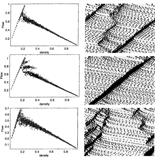
$p_{a}$ and $p_{b}$ are given in Fig. 1. We seesomemetastablebranches in thefundamental diagram.

Moreover,from the spati0-temporal pattern spontaneous jamformationisobserved only if we

allow random braking. Random accerelation alone is not sufficient to produce spontaneous

jamming formation. We also note that a wider scattering area appears if we introduce both

random accerelation and braking.

III. PEDESTRIAN TRAFFIC MODEL

Recent progress in modelling pedestrian dynamics [15] is remarkable and many valuable

results are obtained by using different models, such as the social force model [16] and the

floor field model $[8, 17]$

.

The former model is based _on a system of coupled differential

equations which has to be solved e.g. by using a molecular dynamics approach similar to

the studyof granular matter. Pedestrian interactions are modelled via long-ranged repulsive

forces. In the latter model two kinds of floor fields, i.e., a static and a dynamic one, are

introduced

to translate

a long-ranged

spatial interaction into

an

attractive local interaction,

but

with

memory, similar to the phenomenon ofchemotaxis in biology [18]. It is interesting

that, even though these two models employ different rules for pedestrian dynamics, they

share many properties including lane formation, oscillations of the direction at bottlenecks

[17], and the s0-called faster-is-slower effect [16]. Although these are important basics for

pedestrian modelling, there are still many things to be done in order to apply the models

FIG. 1: Fundamental diagrams and typicalspati0-temporal patternsof the newstochastic Lagrange

model with different value of random parameters. Parameters are set to $V_{\max}=5$ and $S=2.$

Upper two figures are the case of$p_{a}=0$ and $pb$ $=0.2,$ middle ones are$p_{C1}=0.8$ and $pb=0,$ and

the bottom ones are$p_{a}=0.8$ and $pb$ $=0.2.$

this paper, we will propose a method to construct the staticfloor field for complex rooms of

arbitrary geometry. The static floor field is an important ingredient of the model and has

to be specified before the simulations.

First

we

show the update rules of an

extended

floor

field

model for modelling panic

behavior ofpeople evacuatingfrom a

room.

The space is discretizedinto cells ofsize 40

cm

$\cross$

$40$cm which can either beempty or occupied by one pedestrian (hard-core-exclusion). Each

pedestrian

can move

to one of theunoccupiednext-neighborcells $(i,j)$ (orstay at thepresent

cell) at each discrete time step $tarrow t1$ $1$ according to certain transition probabilities

$p_{ij}$

7

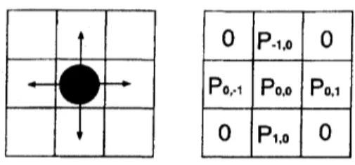
0 $\mathrm{P}.\iota$ 0

$\mathrm{P}_{0}$. Po. $\mathrm{p}_{0.\tau}$

$0$ $\mathrm{P}\tau.0$ 0

FIG. 2: Target cells for a person at the next time step. The von Neumann neighborhood is used

for this model.

For the caseof evacuation processes, the static

_{floor field}

$S$describesthe shortest distance

to

an

exit door. The field strength $S_{ij}$ is set inversely proportional to the

distance

from the

door. The dynamic

_{floor field}

$D$ is a virtual trace left by the pedestrians similar to the

pheromone in chemotaxis [19]. It has its own dynamics, namely diffusion and decay, which

leads to broadening, dilution and finally vanishing of the $\mathrm{t}\mathrm{r}\mathrm{a}\mathrm{c}\mathrm{e}$. At $t=0$ for all sites

$(i,j)$

of the lattice the dynamic field is zero, i.e., $D_{ij}=0.$ Whenever a particlejumps from site

$(i,j)$ to

one

of the neighboring _cells, $D$ at the origin cell is increased by one.

Themodelis able to reproduce various fundamental phenomena, such as lane formation in

a corridor, herding and oscillation at a bottleneck $[8, 17]$. This is an indispensable property

for any reliable model ofpedestrian dynamics, especially for discussing safety issues.

A. Basic update rules

The update rules of our CA have the following structure:

1. The dynamic floor field $D$ is modified according to its diffusion and decay rules,

con-trolled by theparameters$\alpha$ and $\delta$

.

In eachtimestepof thesimulation each single boson

of the whole dynamic field $D$ decays with probability $\delta$ and diffuses with probability

$\alpha$ to one of its neighboring cells.

2. For eachpedestrian, thetransition probabilities$p_{ij}$ for amoveto

an

unoccupied

neigh-bor cell $(i, j)$ are determined by the two floor fields and one’s inertia (Fig. 2). The

values ofthe fields $D$ (dynamic) and $S$ (static)

are

weighted with two sensitivity

pa-rameters $k_{D}$ and $k_{S}$:

with theno rnalization $N$

.

Here_{$p_{I}$} represents the inertia effect [17] given by$p_{I}(i,j)=$ $\exp(k_{I})$ for the direction of one’s motion in the previous time step, and $p_{I}(i,j)=1$

for other cells, where $f\hat{\iota}I$ is the sensitivity parameter. $p\mathfrak{s}v$ is the wall potential which is

explained below. In (17) we do not take into account the obstacle cells (walls etc.) as

well as occupied cells.

3. Each pedestrian chooses randomly a target cell based

on

the transition probabilities

$Pij$

determined

by (17).

4. Whenever two or more pedestrians attempt to move to the

same

target cell, the

move-ment of all

involved

particles is denied with probability $\mu\in[0,1]$, i.e.

all

pedestrians

remain at their site [20]. This means that with probability $1-\mu$

one

of the individuals

movesto the desired cell. Whichone is allowed tomove is decided using aprobabilistic

method $[17, 20]$

.

5. The pedestrians who are allowed to move perform their motion to the target cell

chosen in step

3.

$D$ at the origin cell $(i, 7)$ of each moving particle is increased by

one:

$D_{ij}arrow D_{ij}+1,$ i.e. $D$ can take any non-negative integer value.

The above rules are applied to all pedestrians at the same time (parallel update).

Some

important details

are

explained in the following subsections.

B. Effect of walls

Peopletend to avoid walking closeto walls andobstacles. This can be taken into account

by using “wall

potentials”

-

We introduce

a repulsive potential inverselyproportional to the

distance from the walls. The effect ofthe static floor field is then modified by a factor (see

eq. (17)$)$:

$p_{W}= \exp(k_{W}\min(D_{\max}, d))$, (18)

where $d$ is theminimumdistance from all the walls, and _$kw$ is a sensitivityparameter. The

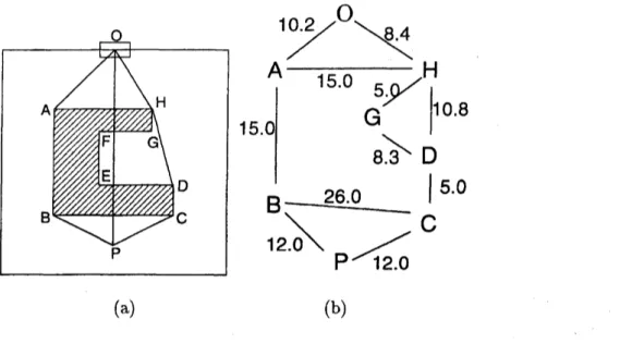
$\mathrm{o}$ $\mathrm{H}$ $\mathrm{A}$ $\nearrow \mathrm{E}\mathrm{F}$ $\mathrm{G}$ $\mathrm{D}$ $\mathrm{B}$ $\mathrm{c}$ $\mathrm{P}$ $10.2\nearrow^{\mathrm{O}}\backslash 8.4$

A

$-\mathrm{H}$

_15.0 $15.0|$ $\mathrm{G}8.35.\backslash \mathrm{D}|10.8$

26.0

$|5.0$ $\mathrm{B}12.0\backslash \mathrm{P}1$ $\mathrm{C}$ (a) (b)

FIG. 3: Example for the calculation of the static floor field using the Dijkstra method, _{(a) A}

room with one obstacle. The door is at $O$ and the obstacle is represented by lines $\mathrm{t}$ –H. (b)

The visibility graph for this room. Each node connected by a bond is

_{“visible”:}

i.e., there are no

obstacles between them. The real number on each bond represents the distance between them as

an illustration.

C. Calculation of the static field in arbitrary geometries

In thefollowing we propose a combination of the visibility graph and Dijkstra’s algorithm

to calculate the static floor field. These methods enable us to determine the minimum

Euclidian $(L^{2})$ distanceof any cell to a door with arbitrary obstacles between them.

Let us explain the main idea of this method by using the configuration given in Fig. $3(\mathrm{a})$

where there isanobstaclein themiddleoftheroom. We will calculate the minimumdistance

between a cell $P$ and the door $O$ by avoiding the obstacle. If the line $PO$ does not cross the

obstacle $A-H,$ then the length of the line, ofcourse, gives the minimum. If, however, asin

the example given in Fig. $3(\mathrm{a})$, the line $PO$ crosses the obstacle, one has to make a detour

around it. Then we obtain two candidates for the minimum distance, i.e., lines

PBAO

and

PCDHO.

The shorter one finally gives the minimum distance between $P$ and $O$

.

Ifthere

are more than one obstacle in the room, then we apply the

same

procedure to each ofthem

repeatedly. Here it is important to note that all the lines pass only the obstacle’s edges with

an acute angle. It is apparent that the obtuse edges like $E$ and $F$ can never be passed by

10

To incorporate this idea into the computerprogram, wefirst need the concept of the

vis-ibility graph in which only the nodes that are visible to each other are bonded [21] ( visible

means here that there are no obstacles between them). The set of nodes consists of a cell

point $P$, a door $O$ and all the acute edges in the

room.

In the case of Fig. $3(\mathrm{a})$, the node

set is $\{P, O, A, B, C, D, G, H\}$ and the bonds are connected between $A-B$, $A-H,$ and so

on

(Fig. $3(\mathrm{b})$).

Each bond has

its own

weight

which corresponds to the Euclidian distance

between them.

Once

we have the visibility graph, we can calculate the distance between $P$ and

0

by

tracing and adding the weight ofthe bonds between them. There are several possible paths

between $P$ and 0, and the

one

with minimum total weight represents the shortest route

between them. The optimization task is easily performedby using the Dijkstramethod [21]

which enables us to obtain theminimum path on a weighted graph.

Performing this procedure for each cell in the room, the method allows us to determine

the

static

floor field for arbitrary

geometries.

D. Simulations: Inertia effect

We focus on measuring the total evacuation timeby changing the parameters $ks$,$f_{\vee D}^{n}$,$k_{I}$, $\mu$

and theconfiguration of theroom, such as width, position and number of doors and obstacles.

In allsimulations we put $D_{\max}=10$, $\alpha=0.2$ and $\delta=0.2,$ and von Neumann neighborhoods

are used in eq. (17) for simplicity. The sizeofthe room is set to 100 $\cross 100$ cells. Pedestrians

try to keep their preferred velocity and direction

as

long as possible. This

is taken

into

account by adjusting the parameter $k_{I}$

.

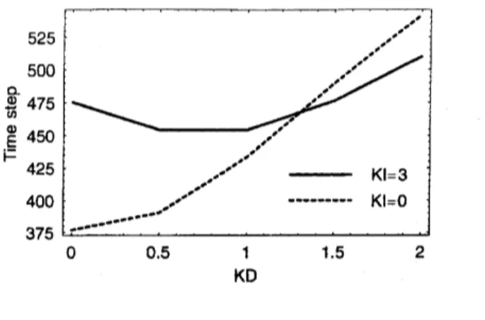
In Fig. 4, total evacuation times from a room

without any obstacles are shown as function of $k_{D}$ in the cases $k_{I}=0$ and $k_{I}=3.$ We

see that it is monotonously increasing in the case $k_{I}=0,$ because any perturbation from

other people becomes large if$f_{\vee D}^{\wedge}$ increases, which causes the deviation from the minimum

route. Introduction of inertia effects, however, changes this property qualitatively

as

seen

in Fig. 4. The minimum time appears around $k_{D}^{\wedge}=1$ in the case $k_{I}=3.$ This is well

explained by taking into account the physical meanings of $k_{I}$ and $k_{D}$. If $f_{\vee I}^{\wedge}$ becomes large,

people become less

flexible

and all of them try to keep their own

minimum

route to

the

exit

according to the static floor field regardless of congestion. By increas$\mathrm{i}_{1\mathrm{l}}\mathrm{g}k_{D}$, one begins to

11

$\Phi \mathrm{f}D\Phi 0_{-}$

KD

FIG. 4: Total evacuation time versus coupling $k_{D}$ to the dynamic floor field in the dependence of

$k_{I}$

.

The room is a simple square without obstacles and 50 simulations are averaged for each data

point. Parameters are $\rho=0.03$,$ks=2$,$kw=0.3$ and $\mathrm{p}$ $=0.$

makes one flexible and hence contributes to avoid congestion. Large $k_{D}$ again works as

strong perturbation as in the case of $k_{I}=0,$ which diverts people from the shortest route

largely. Thus we have the minimum time at a certain magnitude of $k_{D}$, which will depend

on the value of $k_{s}$ and $k_{I}$.

$\mathrm{I}\mathrm{V}$

.

ANT TRAIL MODEL

The ants communicate with each other by dropping a chemical (generically called

pheromone) on the substrate as they crawl forward $[19, 22]$. Although we cannot smell

it, the trail pheromone sticks to the substrate long enough for the other following

sniff-ing ants to pick up its smell and follow the trail. Ant trails may serve different purposes

(trunk trails, migratory routes) and may also be used in a different wayby different species.

Therefore one-way trails are observed as well as trails with counterflow ofants.

In [6] we developed a particle-hopping model, formulated in terms of stochastic CA [2],

which may be interpreted as a model of unidirectional flow in an ant-trail. As in ref. [6],

rather than addressing the question of the

emergence

of the ant-trail, we focus attention

here on the traffic of ants on a trail which has already been formed. Furthermore we have

assumed unidirectional motion. The effects of counterflow, which are important for some

species, will be investigated in the future.

12

$\cap^{9}$ $\cap \mathrm{Q}$ $r^{\mathrm{q}}\backslash$

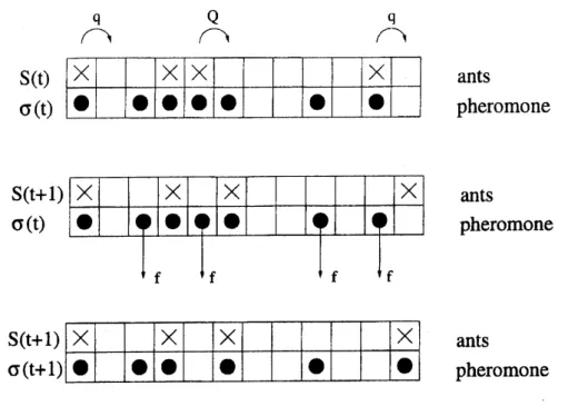
$\mathrm{S}(\mathrm{t})$ ants $\sigma(\mathrm{t})$ pheromone ants pheromone ants pheromone

FIG. 5: Schematic representation of typical configurations; it also illustrates the update procedure.

Top: Configuration at time $t$, i.e.

before

stage I of the update. The non-vanishing hopping

prob-abilities of the ants are also shown explicitly. Middle: Configuration

_after

one possible realisation

of stage $I$. Two ants have moved compared to the top part of thefigure. Also indicated are the

pheromones that may evaporate in stage $II$ of the update scheme. Bottom: Configuration

after

one possible realization of stage II. Two pheromones have evaporated and one pheromone has

been created due to the motion ofan ant.

at most one ant at a time (see Fig. 5). The lattice sites are labelled by the index $i$

$(i=1,2, \ldots, L);L$ _being the length of the lattice. We associate two binary variables $S_{i}$

and $\sigma_{i}$ with each site

$i$ where Si takes the value 0 or 1 depending on whether the cell is

empty or occupied by an ant. Similarly, $\sigma_{i}=1$ if the cell $i$ contains pheromone;

other-wise, $\sigma_{i}=0.$ Thus, we have two subsets of dynamical variables in this model, namely,

$\{S(t)\}\equiv(S_{1}(t), S_{2}(t)$,$\ldots$:$S_{j}(t)$,$\ldots$,$S_{L}(t))$ and $\{\sigma(t)\}\equiv(\sigma_{1}(t), \sigma_{2}(t)$, $\ldots$:

$\sigma_{i}(t)$,

$\ldots$,$\sigma_{L}(t))$. The

instantaneous state (i.e.,the configuration) of the system at any time is specified completely

by the set $(\{S\}, \{\sigma\})$.

Since a unidirectional motion is assumed, ants do not move

backward.

Their

forward-hopping probability is higher if it smells pheromone ahead ofit. The state of the system is

updated at each time step in two stages. In stage I ants are allowedto

move.

Here the subset

13

time $t$.

Stage

II corresponds to the evaporation ofpheromone.

Here

only

the subset

_{$\{\sigma(t)\}$}

is updated so that at the end of

stage

II the new configuration $(\{S(t+1)\}, \{\sigma(t+-1)\})$ at

time $t+1$ is obtained. In each stage the dynamical rules are applied _in parallel to all ants

and pheromones, respectively. Stage $I$: Motion

of

ants

An ant in cell $i$ that has an empty cell in front of it, i.e., _{$S_{i}(t)=1$} and

$S_{i+1}(t)=0,$ hops forward with probability $=\{$ $Q$ if $\sigma_{i+1}(t)=1,$ $q$ if $\sigma_{i+1}(t)=0,$ (19)

where, to be consistent with real ant-trails, we assume $q<Q.$

Stage $II.\cdot$ Evaporation

of

pheromones

At each cell $i$ occupied by an ant after stage I a pheromone will be created, i.e.,

$\sigma_{i}(t+1)=1$ if $\mathrm{S}_{\acute{\mathrm{i}}}(t+1)=1.$ (20)

On

the other hand, any ‘free’ pheromone at a site $i$ not occupied by an ant will evaporate

with the probability $f$ per unit time, i.e., if $S_{i}(t+1)=0$, $\sigma_{\dot{\mathrm{a}}}(t)=1,$ then

$\sigma_{i}(t+1)=\{$ 0 with probability

$f$,

1 with probability $1$

-f.

(21)

Note that the dynamics conserves the number $N$ of ants, but not the number of

pheromones.

The

rules can

be written in a compact form

as

the coupled equations

$S_{j}(t+1)=S_{j}(t)+ \min(\eta j-1(t), Sj-1(t),$$1-Sj(t))$

$- \min(\mathrm{t}\mathrm{X}\mathrm{j}(t), S_{j}(t)$, $1-Sj+1(t))$, (22)

$\sigma j(t+1)=\max(Sj(t+1),\min(\sigma j(t), \xi j(t)))$, (23)

where $\xi$ and

7 are stochastic variables defined by $\mathit{5}j(t)$ $=0$ with the probability $f$ and

$\xi j(t)=1$ with l-f, and $\eta j(t)=1$ with the probability$p=q+(Q-q)\sigma j+1(t)$ and $\eta j(t)=0$

14

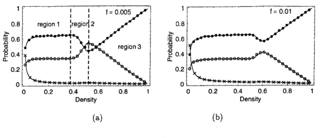
$\mathrm{L}\mathrm{D}\mathrm{D}\iota \mathrm{u}$ $\ovalbox{\tt\small REJECT}^{\mathrm{t}\mathrm{r}\{}$ $\mathrm{n}\varpi\frac{D}{\mathrm{L}}$ $\ovalbox{\tt\small REJECT}$ (a) (b)

FIG. 6: Numerical results for the probabilities offinding an ant(o), pheromone but no ant(o) and

nothing(x) in front ofan ant are plotted against density of the ants. The parametersare $f=$0.005

(in (a)) and $f=0.01$ (in (b)).

A. “Loose” cluster approximation (LCA)

Let us consider again the probabilities $Pa$, $P_{p}$, $P_{0}$ defined in the previous section. For

the purpose of clarifying some subtle concepts of “clustering” we replot these probabilities

for only two specific values of $f$ in Fig. 6; these

data

have been obtained from computer

simulations of our ant-trail model.

There is a flat part of the curves in Fig. 6 in the low density regime; from now onwards,

we shall referto this region as “region 1”. Note that in this region, in spite of low density of

the ants, the probability offinding an ant infront of another is quitehigh. This implies the

fact that ants tend to form a cluster. On the other hand, cluster-size distribution, obtained

from ourcomputer simulations, shows that the probability offinding isolated ants arealways

higher than that of finding a cluster of ants occupying nearest-neighbor sites[23].

These two apparently contradictory observations can be

reconciled

by assuming that the

ants form “loose” clusters in the region 1. The term “loose” meansthat there are smallgaps

in between successive ants in the cluster, and the cluster looks likean usual compact cluster

ifit is seen from a distance (Fig. 7). In other words, a loose cluster isjust a loose assembly

of isolated ants. Thus it corresponds to a space region with densitylarger than the average

density $\rho$, but smaller than the maximal density $(\rho=1)$ of a compact cluster.

1

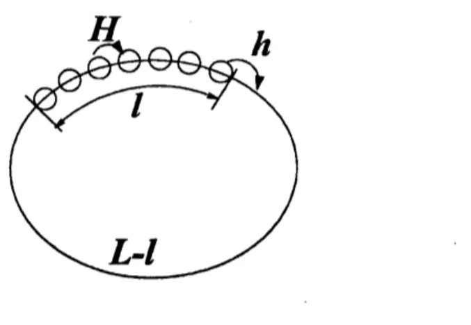
$\mathrm{s}$

FIG. 7: Schematic explanation of the loose cluster. $H$is the hopping probability of ants inside the

loose cluster and $h$ is that of the leading ant.

Then the hopping probability of all the ants, except the leading one, is assumed to be $H$,

while that of the leading one is $h$ (see Fig. 7); the values of _$H$ and $h$ are determined

self-consistently. Before

beginning

the detailed analysis, let

us

consider the properties of $H$ and

$h$. If _$f$ is small enough, then $H$ will be close to $Q$ because the gap between ants is quite

small. On the other hand, if the density of ants is low enough, then $h$ will be very close to

$q$ because the pheromone dropped by the leading ant would evaporate when the following

ant arrives there.

Next we determine the typical size ofthe gap between successive ants in the cluster. We

will estimate this by considering a simple time evolution beginning with an usual compact

cluster (with local density $\rho=1$) without any gap in between the ants. Then the leading

ant willmove forward by one site overthe timeinterval $1$/h. This hopping occurs repeatedly

and in the interval of the successive hopping, the number of the following ants which will

move one step is $H/h$. Thus, in the stationary state, strings (compact _clusters) of length

$H/h$, separated from each other by one vacant site, will produced repeatedly by the ants

(see Fig. 8). Then the average gap between ants is

$\frac{(\frac{H}{h}-1)\cdot 0+11}{H/h}=\frac{h}{H}$, (24)

which is independent of the density $\rho$ of ants. Interestingly, the density-independent

aver-age gap

in the

LCA

is consistent with the flat part (i.e.,

region

1) observed in computer

simulations (Fig. 6). In other words, the region 1 is dominated by loose clusters.

18

$\mathrm{O}$ $\mathrm{O}$

FIG. 8: The stationary loose cluster. The average gap between ants becomes $h/H$, which is

irrelevant to the density of ants.

hopping probability of leading ants becomes large and the

gap

becomes wider,

which

will

increase the flow. We call this region as region 2, in which the “looser” cluster is formed in

the stationarystate. It can becharacterizedby anegative gradient of the density dependence

of the probability to find an ant in front of a cell occupied by an ant (see Fig. 6).

Considering thesefacts, we finallyobtain the following equations for $h$ and $H$:

$( \frac{h-q}{Q-q})^{h}=(1-f)^{L-l}$, $( \frac{H-q}{Q-q})^{H}=(1-f)^{\frac{h}{H}}$, (25)

where

1

is the length of the cluster given by

$l= \rho L+(\rho L-1)\frac{h}{H}$, (26)

and $\rho$ and $L$ are density and the system size, respectively. These equations can be applied

to the region 1 and $\underline{?}$, and solved simultaneously by the Newton method.

Total flux in this system is then calculated as follows. The effective density peff in the

loose cluster is given by

$\rho_{\mathrm{e}\mathrm{f}\mathrm{f}}=\frac{1}{1+h/H}$

.

(27)

Therefore, considering the fact that there are no ants in the part of the length $L-l,$ total

flux $F$ is

$F=$

;

$f(H, \mathrm{t}_{\mathrm{e}\mathrm{f}\mathrm{f}})$, (28)

where $f(H,\rho_{\mathrm{e}\mathrm{f}\mathrm{f}})$ is given by

$f(H, \rho_{\mathrm{e}\mathrm{f}\mathrm{f}})=\frac{1}{2}(1-\sqrt{1-4H_{\beta \mathrm{e}\mathrm{f}\mathrm{f}}(1-\rho_{\mathrm{e}\mathrm{f}\mathrm{f}})})$ (29)

Above the density 1/2, ants are assumed to be uniformly distributed, in which a kind of

MFA works well. We call this region as region

3.

Thus we have three typical regions in this

17

u-2

$\mathrm{A}2$

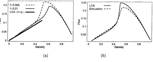
$//’/r’$ IL $\mathrm{I}2$ $\mathrm{A}’\mathrm{r}\mathfrak{n}//$ ty (a) (b)

FIG. 9: (a) Fundamental diagrams of the linear region (bold line) together with numerical results

with parameters $f=$ 0.005 (broken curve) and $f=0.01$ (solid curve). (b) The fundamental

diagram $(f=0.005)$ of the combination ofLCA and (30) (solid curve). The broken curve is the

numerical result for $f=$ 0.005. The system size is $L=350.$

the state is homogeneous. Thus $h$ is determined by

$( \frac{h-q}{Q-q})^{h}=(1-f)^{\frac{1}{\rho}-1}$, (30)

which is the same as our previous paper, and flux is given by $f\cdot(h, \rho)$. It is noted that ifwe

put $\rho=1/2$ and $H=h,$ then (25) coincides with (30).

We

can

focus on the region 1 by assuming $h=q$ in (25). Under this assumption, we

can easily

see

that the flux-densityrelation becomes linear. In Fig. $9(\mathrm{a})$, the two theoretical

lines are almost the same, and the gradientof numerical results are also similar among these

values of$f$, which is quite similar to the theoretical one. In Fig. $9(\mathrm{b})$, the results obtained

from (25) in the region $\rho\leq 1/2$ are shown. Above this value of density, equation (30) is

18

Acknowledgments

The author wishes to acknowledge J.Matsukidaira, A.Schadschneider, A.Kirchner and

D.Chouwdhury for collaborations of studying

CA

models presented in this paper.

[1] B. Chopard and M. Droz, CellularAutomata Modeling

_of

Physical Systems (Cambridge

Uni-versity Press, Australia, 1998).

[2] S. Wolfram, Theory and applications

_of

cellularautomata (World Scientific, Singapore, 1986).

[3] D. Chowdhury, L. Santen, and A. Schadschneider, Phys. Rep. 329, 199 (2000).

[4] D. Helbing, Rev. Mod. Phys. 73, 1067 (2001).

[5] D. Helbing, H. Herrmann, M. Schreckenberg, and D.E.Wolf,

_Traffic

and Granular Flow ’_$gg$

(Springer-Verlag, Berlin, 2000).

[6] D. Chowdhury, V. Guttal, K. Nishinari, and A. Schadschneider, J. Phys. $\mathrm{A}$:Math. Gen. 35,

L573 (2002).

[7] M. Burd, D. Archer, N. Aranwela, and D. J. Stradling, American Natur. 159, 283 (2002).

[8] A. Kirchner and A. Schadschneider, Physica A 312, 260 (2002).

[9] K. Nagel and M. Schreckenberg, Journal of Physics I France 2, 2221 (1992).

10] M. Fukui and Y. Ishibashi, J. Phys. Soc. Jpn. 65, 1868 (1996).

11] K. Nishinari and D. Takahashi, J. Phys. A. 31, 5439 (1998).

12] T. Tokihiro, D. Takahashi, J. Matsukidaira, and J.Satsuma, Phys. Rev. Lett. 76, 3247(1996).

13] T. Musya and H. Higuchi, J. Phys. Soc. Jpn. 17, 811 (1978).

14] K. Nishinari and D. Takahashi, J. Phys. A. 33, 7709 (2000).

15] M. Scheckenberg and S. Sharma, Pedestrian and Evacuation Dynamics (Springer-Verlag,

Berlin, 2001).

16] D. Helbing, I. Farkas, and T. Vicsek, Nature 407, 487 (2000).

17] C. Burstedde, K. Klauck, A. Schadschneider, and J. Zittartz, Physica A 295, 507 (2001).

18] E. Ben-Jacob, Contemp. Phys. 38, 205 (1997).

19] A. Mikhailov and V. Calenbuhr, From Cells to Societies (Springer-Verlag, Berlin, 2002).

20] A. Kirchner, K. Nishinari, and A. Schadschneider, Phys. Rev. $\mathrm{E}67$, 056122 (2003).

21] M. de Berg, M. van Kreveld, M. Overmars, and O. Schwarzkopf, Computational geometry

[2] S. Wolfram, Theory and applications

_of

cellularautomata (World Scientific, Singapore, 1986).

[3] D. Chowdhury, L. Santen, and A. Schadschneider, Phys. Rep. 329, 199 (2000).

[4] D. Helbing, Rev. Mod. Phys. 73, 1067 (2001).

[5] D. Helbing, H. Herrmann, M. Schreckenberg, and D.E.Wolf,

_Traffic

and Granular Flow ’_$gg$

(Springer-Verlag, Berlin, 2000).

[6] D. Chowdhury, V. Guttal, K. Nishinari, and A. Schadschneider, J. Phys. $\mathrm{A}$:Math. Gen. 35,

L573 (2002).

[7] M. Burd, D. Archer, N. Aranwela, and D. J. Stradling, American Natur. 159, 283 (2002).

[8] A. Kirchner and A. Schadschneider, Physica A312, 260 (2002).

[9] K. Nagel and M. Schreckenberg, Journal of Physics I France 2, 2221 (1992).

10] M. Fukui and Y. Ishibashi, J. Phys. Soc. Jpn. 65, 1868 (1996).

11] K. Nishinari and D. Takahashi, J. Phys. A. 31, 5439 (1998).

12] T. Tokihiro, D. Takahashi, J. Matsukidaira, and J.Satsuma, Phys. Rev. Lett. 76, 3247(1996).

13] T. Musya and H. Higuchi, J. Phys. Soc. Jpn. 17, 811 (1978).

14] K. Nishinari and D. Takahashi, J. Phys. A. 33, 7709 (2000).

15] M. Scheckenberg and S. Sharma, Pedestrian and Evacuation Dynamics (Springer-Verlag

Berlin, 2001).

16] D. Helbing, I. Farkas, and T. Vicsek, Nature 407, 487 (2000).

17] C. Burstedde, K. Klauck, A. Schadschneider, and J. Zittartz, Physica A295, 507 (2001).

18] E. Ben-Jacob, Contemp. Phys. 38, 205 (1997).

19] A. Mikhailov and V. Calenbuhr, From Cells to Societies (Springer-Verlag, Berlin, 2002).

20] A. Kirchner, K. Nishinari, and A. Schadschneider, Phys. Rev. $\mathrm{E}67$,056122 (2003).

I9

(Springer-Verlag, Berlin, 1997).

[22] E. Wilson, The insect societies (Belknap, Cambridge, USA, 1971).

[23] $\mathrm{I}[searrow]’$. Nishinari, D. Chowdhury, and A. Schadschneider, Phys. Rev. $\mathrm{E}67$, 036120 (2003).

APPENDIX: THE PAINLEVE 2 EQUATION AND ITS APPLICATION

In this appendix, application of the Painleve 9 equation to an engineering process is

discussed in order to emphasize the importance of the soliton theory.

Injectingglass fibers inanextruderis an important technology in makingplasticmaterials

in order

to

reinforce

them.

The injected fibers are, however,

sometimes

broken

into

pieces

due to inertial forces in the extruder, which damages the strength of materials. Thus it is

important to consider under which conditions fibers will break. To this purpose, let us first

derive a dynamical equation of a fiber in theextruder. The equationofbalance of moments

is given by

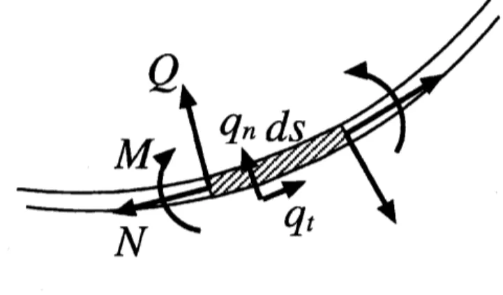
$\frac{\partial NI}{\partial s}=Q,$ (A.1)

where $M=E$Its is the moment and $\kappa$ is the curvature of the fiber (Fig . $Q$ and $s$

are respectively the shearing force and the arc-length of the fiber. Equations of balance of

tangential and transversal force are given by

$\frac{\partial N}{\partial s}+\kappa Q+q_{i}=0$ (A.2)

$- \frac{\partial Q}{\partial s}+\kappa N+q_{n}=0,$ (A.3)

where $N$ is the normal stress and $q_{t}$,$q_{n}$ are the external force acting on the fiber.

20

Eliminating $N$, $Q$ and $\Lambda 1$, we obtain the equation for the curvature as

$\kappa_{ss}=-\frac{\kappa^{3}\sim}{9_{\sim}}-\frac{\kappa^{\sim}}{EI}\int q_{t}ds+\frac{q_{n}}{EI}$. (A.4)

In the extruder it can be shown that we can put both $q_{t}$ and $q_{n}$ as a constant. Thus

(A.4)

which is nothing but the P2 equation. Boundary conditions are

$\kappa(0)=\kappa(L)=0,$ (A.6)

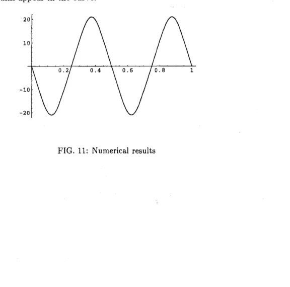
where $L$ is the total length of the fiber, which is usually $\sim$ lOmm. We investigate the P2

equation with the boundary conditions (A.6) numerically. Shooting method is used to adjust

the conditions (A.6). A typical result

are

given in Fig.11. From this figure, we know the

maximum curvature of the fiber. If the maximum exceeds the surrender condition of the

material, then it will break into pieces and the number of pieces may correspond to the

number of extremums appear in the curve.

20

10

0.20.4 0.6 0.8 1

10

20