Probabilistic Construction of Solutions To Some Integral Equations (Symposium on Probability Theory)

Probabilistic

Construction

of

Solutions

To

Some

Integral Equations

Isamu

D\^oku

Department of Mathematics,

Saitama

University

Saitama, 338-8570 Japan

\S 1.

Notations and assumptions

For simplicity, let $D_{0}:=\mathbb{R}^{3}\backslash \{0\}$, and

we

put $\mathbb{R}_{+}:=[0, \infty$). For every

$\alpha,$$\beta\in \mathbb{C}^{3}$, we

use

thesymbol $\alpha\cdot\beta$ for the inner product, and we define

$e_{x}$ $:=x/|x|$

for every $x\in D_{0}$. In this article we consider the following deterministic nonlinear

integral equation:

$e^{\lambda t|x|^{2}}u(t, x)=u_{0}(x)+ \frac{\lambda}{2}\int_{0}^{t}dse^{\lambdas|x|^{2}}\int p(s, x, y;u)n(x, y)dy$

$+ \frac{\lambda}{2}\int_{0}^{t}e^{\lambda s|x|^{2}}f(s, x)d_{\mathcal{S}}$, for $\forall(t, x)\in \mathbb{R}_{+}\cross D_{0}$. (1)

Here$u\equiv u(t, x)$ is an unknownfunction: $\mathbb{R}_{+}\cross D_{0}arrow \mathbb{C}^{3},$ $\lambda>0$, and$u_{0}:D_{0}arrow \mathbb{C}^{3}$

is theinitial data such that $u(t, x)|_{t=0}=u_{0}(x)$

.

Moreover, $f(t, x)$ : $\mathbb{R}_{+}\cross D_{0}arrow \mathbb{C}^{3}$

is.a

given function satisfying $f(t, x)/|x|^{2}=:\tilde{f}\in L^{1}(\mathbb{R}_{+})$. The integrand

$p$ in (1) is given by

$p(l, x, y;u)=u(x, y)\cdot e_{x}\{u(t, x-y)-e_{x}(u(t, x-y)\cdot e_{x}$ ₍₂₎

On the other hand, we consider aMarkov kernel $K$ : $D_{0}arrow D_{0}\cross D_{0}$

.

Actually, for

every $z\in D_{0},$ $K_{z}(dx, dy)$ lies in the space $\mathcal{P}(D_{0}\cross D_{0})$ of all probability measures

on aproduct space $D_{0}\cross D_{0}$. When thekernel $k$ is given by $k(x, y)=i|x|^{-2}n(x, y)$,

then we define $K_{z}$

as

a Markov kernel satisfying that for any positive measurable

function $h=h(x, y)$ on $D_{0}\cross D_{0},$

$\iint h(x, y)K_{z}(dx, dy)=\int h(x, z-x)k(x, z)dx$ ₍₃₎

Moreover, we

assume

that for every measurable functions $f,$$g>0$ on $\mathbb{R}^{+},$

$\int h(|z|)v(dz)\int g(|x|)K_{z}(dx, dy)=\int g(|z|)\nu(dz)\int h(|y|)K_{z}(dx, dy)$ ₍₄₎

\S 2.

Main result

In this section

we

shall state

our

main result, which asserts the existence and

uniqueness of solutions to the nonlinear integral equation (1). As

a

matter of

fact, the solution $u(t, x)$

can

be expressed

as

the expectation of

a

star-product

functional, which is nothing but a probabilistic solution constructed by making

use of thebelow-mentioned branchingparticle systems and branching models. Let

$M_{\star}( \omega)=\prod\star[x_{m}^{-}]^{-}-m^{1}.m_{3}[u_{0}, f](\omega)$, (5)

be

a

probabilistic representation in terms of tree-based star-product functional

with weight $(u_{0}, f)$

.

For the details of the definition,

see

the succeeding sections.

Onthe other hand, $M_{*}^{\langle U,F\rangle}(\omega)$ denotes the corresponding$*$-productfunctionalwith

weight $(U, F)$

.

In fact,

as

to be

seen

in what follows, in

a

similar

manner

as

the

case

of

a

star-product functional

we

can

construct $a(U, F)$-weighted $tree-$based $*-$

product functional $M_{*}^{\langle U,F\rangle}(\omega)$, which is indexed by the nodes _{$(x_{m})$} ofa binarytree.

Herewe suppose that $U=U(x)$ $($resp. $F=F(t, x))$ is a non-negative measurable

function on $D_{0}$ (resp. $\mathbb{R}_{+}\cross D_{0}$) respectively, and also that $F$ x) $\in L^{1}(\mathbb{R}_{+})$

for each $x$

.

Indeed, in construction of the $*$-product functional, the product in

question is taken

as

ordinary multiplication $*$ insteadof the star-product $\star$ in the

definition of star-product functional.

$T$heorem 1. Suppose that _{$|u_{0}(x)|\leq U(x)$}

for

$\forall x$ and _{$|\tilde{f}(t, x)|\leq F(t, x)$}

for

$\forall t,$$x$, and also that

for

some

$T>0$ ( $T>>1$ sufficiently large),

$E_{T,x}[M_{*}^{\langle U,F\rangle}]<\infty$, ae.

$-x$ (6)

Thenthere exists $a(u_{0}, f)$-weighted tree-based star$\star$-product

functional

$M_{\star}^{\langle u_{0},f\rangle}(\omega)$,

indexed by a set

_of

node labels accordingly to the tree structure which

a

binary

crit-ical branching process $Z^{K_{x}}(t)$ determines. Furthermore, the

function

$u(t, x)=E_{t,x}[M_{\star}^{\langle uo,f\rangle}]$ (7)

$give\mathcal{S}$ a unique solution to the integral equation (1). Here $E_{t,x}$ denotes the

expecta-tion with respect to a probability

measure

$P_{t,x}$ as the time-reversed law

of

$Z^{K_{x}}(t)$.

\S 3.

Branching model

Inthis section

we

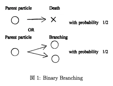
consider a continuous time binary critical branchingprocess

$Z^{K_{x}}(t)$

on

$D_{0}$, whose branching rate is given by a parameter $\lambda|x|^{2}$, whose

branch-ing mechanism is binary with equi-probability, and whose descendant branchbranch-ing

$PaIe\mathfrak{n}t$ particle Death

$O$ $arrow$ $\cross$

with probability 1/2 OR

1/2

図1: Binary Branching

notice of the tree structure which the process $Z^{K_{x}}(t)$ determines,

we

denote the

space of marked trees

$\omega=(t, (t_{m}), (x_{m}), (\eta_{m}), m\in \mathcal{V})$ (8)

by $\Omega$. Furthermore, we write the

time-reversed law of $Z^{K_{x}}(t)$ being

a

probability

measure on $\Omega$ as

$P_{t,x}\in \mathcal{P}(\Omega)$. Here $t$ denotes the birth time of common ancestor,

and theparticle$x_{m}$ dieswhen $\eta_{m}=0$, whileit generates two descendants$x_{m1},$$x_{m2}$

when $\eta_{m}=1$

.

On the other hand,

$\mathcal{V}=\bigcup_{p\geq 0}\{1, 2\}^{\ell}$

is a set of all labels, namely, finite sequences of symbols with length $\ell$, which

describe thewholetree structure given. For$\omega\in\Omega$ we denote by$\mathcal{N}(\omega)$ the totality

of nodes being branching points of tree, and let $N_{+}(\omega)$ be the set of all nodes $m$

being a member of $\mathcal{V}\backslash \mathcal{N}(\omega)$, whose direct predecessor lies in $\mathcal{N}(\omega)$ and which

satisfies the condition $t_{m}(\omega)>0$, and let $N_{-}(\omega)$ be the

same

set as described

above, but satisfying $t_{m}(\omega)\leq 0$

.

Finallywe put

$N(\omega)=N_{+}(\omega)\cup N_{-}(\omega)$. (9)

\S 4.

Star-product functional and $*$-product functional

In what follows we shall intoduce a tree-based star-product functional in

order to construct a probabilistic solution to the class of integral equations (1).

onto its orthogonal part of the $z$ component in $\mathbb{C}^{3}$

, and we define a $\star$-product of

$\beta,$

$\gamma$ for $z\in D_{0}$ as

$\beta\star_{1z]}\gamma=-i(\beta\cdot e_{z})Proj^{z}(\gamma)$. (10)

We shall define $\Theta^{m}(\omega)$ for each $\omega\in\Omega$realized as follows. When $m\in N_{+}(\omega)$, then

$\Theta^{m}(\omega)=\tilde{f}(t_{m}(\omega), x_{m}(\omega))$, while $\Theta^{m}(\omega)=u_{0}(x_{\mathfrak{m}}(\omega))$ if $m\in N_{-}(\omega)$. Then

we

define

$\Xi_{m_{2}^{1}.m_{3}}^{rn}(\omega)\equiv\Xi_{m_{2}^{1},m_{3}}^{m}[u_{0}, f](\omega):=\Theta^{m_{2}}(\omega)\star_{[x_{m_{1}}]}\Theta^{m_{3}}(\omega)$, (11) where as for the product order in the star-product $\star$, when we write $m\prec m’$ lexicographically with respect to the natural order $\prec$, the term $\Theta^{m}$ labelled by _$m$

necessarily occupies the left-hand side and the other $\Theta^{m’}$

labelled by $m’$ occupies the right-hand side by all means. And besides,

as

abuse ofnotation we write

$-m,\emptyset m\equiv_{-,\emptyset[u_{0}}, f](\omega):=\Theta^{m}(\omega)$, (12)

especially when $m\in \mathcal{V}$ is a label of single terminal point in the restricted tree structure in question.

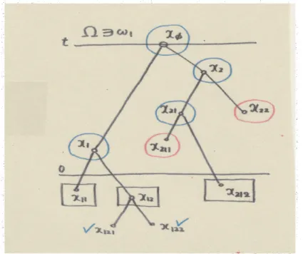
図 2: Example: A realized Tree

Under these circumstances, we considerarandom quantity which obtained by executing the star-product $\star$ inductively at each node in$\mathcal{N}(\omega)$, and we call it a

tree-based $\star$-product functional, and we express it symbolically as

where $m_{1}\in \mathcal{N}(\omega)$ and _{$m_{2},$}$m_{3}\in N(\omega)$, and by the symbol $\prod\star$ (as a product relative to the star-product) we mean that the star-products $\star$’s should be suc-ceedingly executed in a lexicographical manner with respect to $X_{m}^{-}$ such that $\tilde{m}\in$

$\mathcal{N}(\omega)\cap\{|\tilde{m}|=\ell-1\}$ when $|m_{1}|=\ell.$

Example 1. Now letussupposethat atree structure$\omega_{1}(\in\Omega)$ has beenrealized

here (see Figure 2).

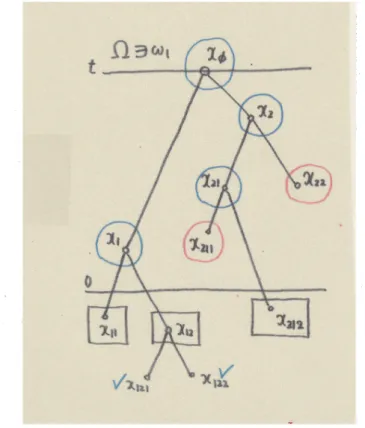
図3: Classification ofNodes

Next

we

shall classify those nodes in the realized tree $\omega_{1}$. As a matter of fact, as

to those two particles located at $x_{11}$ and $x_{12}$ with nodes of the level $|m|=\ell=2$ accompanied by the pivoting node $x_{1}$, we can construct

$-11,121$

byastar-product $u_{0}(x_{11}(\omega_{1}))\star_{[X_{1}]}u_{0}(x_{12}(\omega_{1}))$ inaccordance withthe rule, because both $m_{1}=11$ and $m_{2}=12lie$ in $N_{-}(\omega)$. As to the node _{$x_{21}$}, how to construct $—(\omega_{1})$is thealmostsamething

as

described above. In fact,it goessimilarlybecause

$x_{211}$ lies in $N_{+}(\omega_{1})$ and $x_{212}$ lies in $N_{-}(\omega_{1})$. Accordingto the rule, it follows that

hence $\Xi_{211,212}^{21}(\omega_{1})$ is given by $\tilde{f}(t_{211}(\omega_{1}), x_{211}(\omega_{1}))\star_{[x_{21}]}u_{0}(x_{212}(\omega_{1}))$,

see

Figure 3.

Consequently,

we

obtain finally

$M_{\star}^{\langle u0f\rangle}(\omega_{1})=\cdot(u_{0}(x_{11})\star_{[x_{1}]}u_{0}(x_{12}))\star_{[x_{\phi}]}$

$\{(u(x_{212}))\star_{[x_{2}]}\tilde{f}(t_{22}, x_{22})\}$

.

(14)

口

\S 5.

Outline of proof: tree-based star-product functional

as a

solution

In this section we are first going to construct $a(U, F)$-weighted tree-based

$*$-product functional $M_{*}^{\langle U,F\rangle}(\omega)$,

which is indexed by the nodes $(x_{m})$ of

a

binary

tree. Here recall that $U=U(x)$ $($resp. $F=F(t, x))$ is

a

non-negative measurable

function

on

$D_{0}$ (resp. $\mathbb{R}_{+}\cross D_{0}$) respectively, and also that $F$ $x$) $\in L^{1}(\mathbb{R}_{+})$

for each $x$. Moreover, in construction of the functional, the product is taken

as

ordinary multiplication $*$ instead of the star-product $\star.$

In what follows we shall give

an

outline of the proofof Theorem 1. We need the

following technical lemma, which plays an essential role in the proof.

Lemma 2. For$0\leq t\leq T$ and$x\in D_{0}$, the

function

$V(t, x)=E_{t,x}[M_{*}^{\langle U,F\rangle}(\omega)]$

satisfies

$e^{\lambda t|x|^{2}}V(t, x)=U(x)+ \int_{0}^{t}ds\frac{\lambda|x|^{2}}{2}e^{\lambda s|x|^{2}}\{F(s, x)+\int V(s, y)V(s, z)K_{x}(dy, dz)\}.$

(15)

As

a

matter of fact, the mapping : $[0, T]\ni t\mapsto e^{\lambda|x|^{2}}tV(t, x)\in\overline{\mathbb{R}}_{+}$ is

non-decreasing,

so

that, it proves to be that

$E_{t,x}[M_{*}^{\langle U,F\rangle}(\omega)]<\infty$ (16)

holds for$\forall t\in[0, T]$ and $x\in E_{c}$, where $E_{c}$ is

a

measurableset

on

which the validity

of$E_{t,x}[M_{*}^{\langle U,F\rangle}]<\infty$ maybe kept. Another important aspect for the proof consists

in establishment of the following $M_{*}$-control inequality. That is to say, we have

$|M_{\star}^{\langle u0,f\rangle}(\omega)|\leq|M_{*}^{\langle U,F\rangle}(\omega)|$ (17)

because of the validity ofa simple inequality

$|w\star_{[x]}v|\leq|w|\cdot|v|$ for $w,$$v\in \mathbb{C}^{3}$ and $x\in D_{0}.$

On the other hand, it is derived that the space of solutions to (1) is formed by the

condition

A similar discussion

as

above leads to

$u(t, x)=E_{t,x}[M_{\star}^{\langle u_{0},f\rangle}( \omega)]=e^{-\lambda t|x|^{2}}u_{0}(x)+\int_{0}^{t}ds\lambda|x|^{2}e^{-\lambda(t-s)|x|^{2}}\cross$

$\cross\frac{1}{2}\{\tilde{f}(s, x)+\iint E_{s,x_{1}}[M_{\star}]\star_{[x]}E_{s,x_{2}}[M_{\star}]K_{x}(dx_{1}, dx_{2})\}$ . (18)

Finallywe

can

deduce that $u(t, x)=E_{t,x}[M_{\star}^{\langle u0,f\rangle}(\omega)]$ satisfies the integral equation

(1), and this $u(t, x)$ _is

a

solution lying in the space $\mathcal{D}$

.

Actually, $\mathcal{D}$

is a space of

all functions $\varphi$ : $\mathbb{R}_{+}\cross D_{0}arrow \mathbb{C}^{3}$, being continuous in $t$ and measurable such that

$\int_{0}^{\infty}d_{\mathcal{S}}\int|p(s, x, y;\varphi)|K_{x}(dy, dz)<\infty$, ae. _$-x.$

Acknowledgements

This work is supported in part by Japan MEXT Grant-in-Aids SR(C) 24540114

and also by ISM Coop. Res. Program: 2011-CRP-50I0.

References

[1] Aldous, D. The continuum randomtree I.

&

III. Ann. Probab. 19 (1991), 1-28;

ibid. 21 (1993), 248-289.

[2] Aldous, D. Tree-based models for random distribution of

mass.

J. Stat. Phys.

73

(1993), 625-641.

[3] Aldous, D. and Pitman, J. Tree-valued Markov chains derived from

Galton-Watson processes. Ann. Inst. Henri Poicar\’e 34 (1998),

637-686.

[4] Aldous, D. and Pitman, J. Inhomogeneous continuum random trees and the

entrance boundary of the additive coalescent. Probab. Theory Relat. Fields

118 (2000), 455-482.

[5] Chauvin, B., Klein, T., Marckert, J.-F. and Rouault, A. Martingales and profile

of binary search trees. Electr. J. Probab. 10 (2005), 420-435.

[6] Drmota, M. Random $\mathcal{I}\succ ees$

.

Springer, Wien, 2009.

[7] Evans, S.N. Probability and Real Trees. Lecture Notes in Math. vol.1920,

Springer, Berlin, 2008.

[8] Harris, T.E. The Theory

_of

Branching Processes. Springer, Berlin, 1963.

[9] Le Gall, J.-F. Random trees and applications. Probab. Survey. 2 (2005), 245-311.