FitzHugh-Nagumo方程式に現れる微細パターンについて (反応拡散系におけるパターン形成と漸近的幾何構造の研究)

FitzHugh-Nagumo 方程式に現れる微細パターンについて

東京大学大学院数理科学研究科 大下承民 (Yoshihito Oshita)

Graduate School of Mathematical Sciences, University ofTokyo

1

Introduction

FitzHugh-Nagumo equation was introduced as a reduced equation of Hodgkin-Huxley model, which describespropagation of signals alonga

nerve

axon.

Ithas turned out to be related to the theory ofthe pattern formation in mathematical biology and

wave propagation in excitable media. Refer to [2, 3, 5, 6, 7, 8]. FitzHugh-Nagumo equation is a system of reaction-diffusion equation consisting of two unknown func-tions $u$ and $v$ representing concentrations of activator and inhibitor respectively, and

typically of the form

$u_{t}=\epsilon^{2}\Delta u$ _{$+f(u)-\kappa v,$}

$(E- 1)_{\epsilon}$ in $El$ $\mathrm{x}\mathbb{R}_{+}$

$\tau v_{t}=D\Delta v+u-m-\gamma v,$

with the homogeneous Neumann boundary condition

on

90, where $\Omega\subset \mathbb{R}^{N}$ is

a

bounded domain; $f(u)=-\mathrm{I}\mathrm{I}\mathrm{f}(\mathrm{u})$ ($W\in C^{2}(\mathbb{R})$ is a double-well potential which has

global minima exactly at $\mathrm{f}1$, and $W(\pm 1)=0)$ isa bistable nonlinearity; $m\in(-1, +1)$

is a constant; $\kappa$,$\tau$,$D$ and $\mathrm{y}$ are positive constants and $\epsilon$ is a positive parameter.

Throughout this survey we always impose the homogeneous Neumann boundary

con-dition. We study the parameter scaling $\epsilon$ $arrow$p 0 in $(E- 1)_{\epsilon}$

.

We also study the following

scaling.

$u_{t}=\epsilon^{2}\Delta u+$ $\mathrm{j}(u)$

$- \frac{\epsilon}{\mu}v$,

(E-1)$\cdot$ in 0 $\mathrm{x}\mathbb{R}_{+}$

$\tau v_{t}=D\Delta v+-$_{$u-m-\gamma v,$}

where $\mu$,$\tau$,$D$ and $\mathrm{y}$ are positive constants and $\epsilon(arrow 0)$ is apositive parameter. In

addition,

we

study another scaling, that is, $u_{t}=\epsilon^{2}\Delta u+$ $\mathrm{j}(\mathrm{t}\mathrm{z})$

$- \frac{\epsilon}{\mu}v$,

$(E-3)_{\epsilon,D}$ in $\Omega\cross \mathbb{R}_{+}$

83

where $\mu$, $\mathrm{r}$ and

$\mathrm{y}$ are positive constants and $\epsilon(arrow 0)$ and $D(arrow\infty)$

are

positive

parame-ters. Stationarysolutions of$(E- 1)_{\epsilon}$

are

functions _$u$, $?\mathrm{J}$which satisfy thefollowing system

of elliptic equations

(1) $\epsilon^{2}\Delta u+f(u)-\kappa v$ _{$=0,$ in Q.}

$D\Delta v+u-m-\gamma v=0,$

Similarly the stationary _solutions of $(E- 2)_{\epsilon}$ and $(E- 3)_{\epsilon,D}$ solve

(2) $\epsilon^{2}\Delta u+f(u)-$

$\mathit{7}$

$v=0,$

in $\Omega$

.

$D\Delta v+-$_{$u-m-\gamma v=0,$}

Note that these equations

are

independent of the constant $\tau$

.

It is easy to see that if $u$,$v$ solves (1), then $u$ is a critical point ofthe functional $I_{\epsilon}$ defined by

$I_{\epsilon}[u]= \int_{\Omega}\frac{\epsilon^{l}}{2}|\nabla u|^{2}+W(u)+\frac{D\kappa}{2}|\nabla(T(u-m))|^{2}+\frac{\kappa\gamma}{2}\{T(u-m)\}^{2}dx$_, $u\in H^{1}.(\Omega)$,

where $T=(-D\Delta+\gamma)^{-1}$ is the Green _{operator of} $-Di^{\mathit{5}}$ _$+\gamma$ with the homogeneous

Neumann boundary condition. We remark that if $\tau=0$

were

satisfied, the _activator

of $(E- 1)_{\epsilon}$, $u(\cdot, t)$ would be the gradient flow of

$I_{\epsilon}$

.

However since

$\tau>0,$ the activator $u(\cdot, t)$ of$(E- 1)_{\epsilon}$ is different from a gradient flow of

$I_{\epsilon}$

.

In case of _{$(E- 2)_{\epsilon}$}

and $(E-3)_{\epsilon,D}$,

we deal with the functionate $J_{\epsilon}$ and $J_{\epsilon}$

,$D$ respectively defined as follows:

$J_{\epsilon(,D)}[u]= \int_{\Omega}\frac{\epsilon^{l}}{2}|$Vu$|^{2}+$

W{u)

_{$+ \frac{D\epsilon}{2\mu}|\nabla(7(u-m))|^{2}+\frac{\epsilon\gamma}{2\mu}\{T(u-m)\}^{2}dx$}

.

(Note that the operator $T$ depends

on

_$D.$) It is easy to

see

that the family of the $\mathrm{f}$

nc-tionals $I_{\epsilon}$ and

$J_{\epsilon(,D)}$ admit a global minimizer for each parameter. We

are

concerned with the asymptotic behavior of _{such minimizers for each parameter-scalings stated} above. (For the stability, refer to [13].)

The homogenization problems_{with twolengthscales have been studiedrecently (refer} to [1, 4, 9]$)$

.

Also refer to [10, 12, 15] for the problem related

to diblock copolymer. We

assume

that $f$ has polynomial growth at infinity and has three

zeros:

-1,

$a$,1

2

Statement of Main

Results

To state thefirstresult,

we use

the notionofYbungmeasure, ausefultoolforstudying

a

sequence of functions which is oscillating and not convergent. We use the Young

measure

which is a map ffom $\Omega$ to the set of all probability

measures

on R. A usual

function $u(x)$ corresponds to the family of Dirac

measures

$\delta_{u(x)}$

.

The fundamental

theorem for Young

measure

states the sufficient condition for relative compactness of asequence of Young

measures

in an appropriate topology. We can get the limit Young

measure

instead of the limit function. (Refer to [14].) In order to state the main result, define the constant

$c_{o}= \frac{\sqrt{2}}{\int_{-1}^{1}\sqrt{W(s)}ds}$

and the set of all admissible functions in the limiting problem which

we

will obtain later,

$\mathcal{G}(\Omega)=$

{tz

$\in BV(\Omega);.|\mathrm{t}\mathrm{z}(x)|=1$ for almost all $x\in\Omega$

},

$\mathcal{M}(\Omega)=$

{tz

$\in \mathcal{G}$; $\langle u)_{0}=m$

}.

Here $\langle\cdot\rangle_{\Omega}$ denotes the average on $\Omega$

.

We

use

the following notation: Pq(G) denotes the

perimeter of$G\subset\Omega$ with respect to $\Omega$

.

Theorem 2.1. The following statements hold:

(i) For any$\epsilon$ $>0,$ there exists a stable stationary solution $(u_{\epsilon}, v_{\epsilon})$

of

$(E- 1)_{\epsilon}$ such that

for

any sequence $\epsilon_{n}arrow 0,$ $u_{\epsilon_{n}}$ is not convergent in $L^{1}(\Omega)$ andgenerates Young

measure

$\nu=(\nu_{x})_{x\in\Omega}$ with $\nu_{x}=\frac{1-m}{2}\delta_{-1}+\ovalbox{\tt\small REJECT} 12$$\delta_{1}$

for

almost all$x\in\Omega$

.

(ii) For any sequence $\epsilon_{n}arrow 0,$ there exists a subsequence $\epsilon_{k}=\epsilon_{n_{k}}$ and stable

station-ary solutions $(u_{k}, v_{k})$

of

$(E- 2)_{\text{\’{e}}_{k}}$ such that_{$u_{k}$} converges strongly in $L^{1}(\Omega)$ to a solution

of

$(P)^{\mu}$ _{$\min_{u\in \mathcal{G}}B^{\mu}(u)$}, $B^{\mu}(u)= \frac{2}{c_{0}}P_{\Omega}(\{u=1\})+\frac{1}{2\mu}\int_{\Omega}(u-m)T(u-m)dx$

.

(iii) For any sequence$\epsilon_{n}arrow 0$,$D_{n}arrow\infty$, there $e$$\dot{m}t$ subsequences

$\epsilon_{k}=\epsilon_{n_{k}}$,$D_{k}=D_{n_{k}}$

85

property that $u_{k}$ converges strongly in $L^{1}(\Omega)$ to a solution

of

$(\overline{P})^{\mu}$

$\min_{u\in \mathcal{G}}\tilde{B}(u)$, $\overline{B}(u)=\frac{2}{c_{0}}P_{\Omega}(\{u=1\})+\frac{1}{2\mu\gamma}|\Omega|(\langle u\rangle-m)^{2}$

.

Note that the solutions in Theorem 2.1 (i) do not have a limit. In fact, from the result of [11], for $(E- 1)_{\epsilon}$, any stationary solutions which has asmooth surface

as a

limit

must be unstable. In Theorem 2.1, we obtained the two limiting problems, $(P)^{\mu}$ and

$(\tilde{P})^{\mu}$, which

are

the geometric

minimization problem with a parameter dependence, and determine thelocation of interiorboundary layers. The next theorem

concerns

the asymptotic _{behavior of solutions of the two problems} $(P)^{\mu}$ and $(\tilde{P})^{\mu}$

as

$72arrow 0.$

Theorem 2.2. The following statements hold: (i) Let $u^{\mathrm{j}}$

be a solution

_of

$(P)^{\mu}$

.

Then

for

any sequence

$\mu_{k}arrow$p 0, $u^{\mu}$ generates the

same

Young

measure

$\nu$ as in Theorem 2.1 (i).

(ii) Let $u$\overline P be a solution

of

$(\tilde{P})^{\mu}$. Then

for

any sequ

ence

$\mu_{n}arrow 0,$ there exists $a$

subsequence $\mu_{k}=\mu_{n_{k}}$ such that $\overline{u}^{\mu k}$ converges

strongly in $L^{1}(\Omega)$ to a solution _$u$’

of

$\min_{u\in\Lambda 4}7’ \mathrm{g}(\{u=1\})$,

and generates the Young

measure

$\nu=(\nu_{x})_{x\in\Omega}$ with $\nu_{x}=\delta_{u^{*}(x)}$

for

almost all $x\in\Omega$

.

Note that for the problem $(P)^{\mu}$, we obtained a similar result as Theorem 2.1 (i),

which corresponds to the case $\epsilon$

$=\mu\kappa$

.

We see that

we can

construct a sequence of

solutions for $(E- 2)_{\epsilon}$ which converges to

a

pattern with an

arbitrary large perimeter if

we

choose sufficiently small $\mu$

.

In the next Theorem,

we

derive the geometric interfaceequation associated with the solutions of$(P)^{\mu}$ and $(\tilde{P})^{\mu}$

.

We

use

the following

notations: We take the sign of

mean

curvature such thatprincipalcurvature of thesphereis negativewhen the normal vector points to the center, $\partial’$ denotes the

relative boundary with respect to $\Omega$

.

Theorem 2.3. The

_follow

$.ng$ statements hold:

(i) For

_fixed

$\mu>0,$ let $u$ be a solution

of

$(P)^{\mu}$ and $\Gamma=\partial’\{u=1\}$

.

Assume that $\Gamma$

is smooth in a neighborhood $U$

of

a point$x_{o}\in\Gamma$. Then there holds

$\mu H=c_{o}T(u-m)$,

on

$\Gamma\cap U,$

where $H$ denotes the mean _{$cu$ vature}

of

$\Gamma$ (when the normal vector points

from

$\{u=$

(ii) For

_fixed

$\mu>0,$ let $\overline{u}$ be a solution

of

$(P)^{\mu}$ and $\Gamma=\partial’\{\overline{u}=1\}$

.

Assume that $\Gamma^{1}$

is smooth in a neighborhood $\overline{U}$

of

a point$\overline{x}_{o}\in\overline{\Gamma}\sim$ Then there holds

$\mu H=\frac{c_{o}}{\gamma}$$(\langle\overline{u}\rangle-772)$ ,

on

$\tilde{\Gamma}\cap\overline{U}$,

where $H$ denotes the mean curvature

of

$\Gamma$ (when the normal vector points

from

$\{\overline{u}=$

$-1\}$ to $\{\overline{u}=1\})$

.

Theorem 2.3 (ii) implies that solutions of $(P)^{\mu}$ typically involve apartition of$\Omega_{-}$into

regions separated by surfaces of a constant mean curvature. In [3], they obtained a

limiting free boundary problem from an Allen-Cahn equation with a nonlocal term,

which arises as a limit of

a

reaction-diffusion system. Then we

see

that any surface which corresponds to stationary solutions of the motion law obtained in [3] has also a

constant

mean

curvature.

3

Remarks

on

Two

Dimensional

Problems

$u\in \mathcal{G}(\Omega)$ is called planar if $?\mathrm{j}$ $=$ $u(x_{1}$,

. .

.

’$x_{N})$, $(x_{1}$,

. . .

’$x_{N})\in\Omega$ depends only on $x_{1}$

.

Proposition 3.1. Let $N=2$ and $\Omega=(0,1)^{2}$

.

Then there exists a constant _$m\in$

(-1,1), sufficiently close to -1, and a sequence $\mu_{k}" \mathrm{p}$ $0$ such that ever_$ry$ solution $u^{\mu k}$

of

$(P)^{\mu k}$ is not planar.

Wethinktypical interfaces for solutionsof$(P)^{\mu}$ shouldbelines

or

circles when$N=2.$

We believe that, for sufficiently close to 1, and $\mu$ small, an interface approximated by

a circle of a small radius, centered

near

the points

on

the boundary, which have the maximum mean curvature, should arise as in Cahn-Hilliard theory.

Figure 1 Typical Patterns; the black part is the region $u\sim 1$ and the white

part is the region $u\sim-1$. (i) the left picture is the case $m<0;(\mathrm{i}\mathrm{i})$ the central

87

We cannot expect that the minimizers of$I_{\xi \mathrm{j}}$ are precisely periodic

in two dimensional arbitrary domain unlike the

one

_{dimensional case. However the Young}

_measure

gen-erated by the global minimizers is constant in $x\in$ D. (See, Theorem 2.1 (i).) This

suggests that the energy of global _{minimizers distribute somewhat uniformly. Then if} the minimizers

are

not planar, what do they look like? In fact, non-planarminimizers which have hexagonal structures are observed (see Figure 1). We would like to give a

mathematical account of this hexagonal pattern selection drawn in Figure 2.

Figure 2 hexagon structure

Since the formal discussion suggests that we should study the pattern of the order

$\epsilon^{1/3}$,

we use the followingscaling and transform$\mathrm{e}\mathrm{d}$ $\mathrm{f}$

nctions

$\hat{\epsilon}=\epsilon^{2/3}$

,$y= \frac{x}{\epsilon^{1/3}}$,

$u(x)=U(y)$,$v(x)=$

\epsilon 273V(y),

$-D\Delta V+\gamma\hat{\epsilon}V=U-m.$

Now let $U$,$V$ be extended to the whole $\mathbb{R}^{N}$ i

$\mathrm{n}$ a symmetric and periodic way with

a periodic unit domain Y. Then if $\{y;\hat{\epsilon}y\in\Omega\}$ is packed with a finite number of

translated $\mathrm{Y}$, we

have

$\epsilon^{-2/3}|\Omega|^{-1}I_{\text{\’{e}}}[u]=$

$\frac{1}{|\mathrm{Y}|}\int_{\mathrm{Y}}\frac{\hat{\epsilon}}{2}|\nabla U|^{2}+\frac{W(U)}{\hat{\epsilon}}+\frac{(\langle U\rangle_{\mathrm{Y}}-m)^{2}}{2\gamma\hat{\epsilon}}+\frac{D\kappa}{2}|\nabla V|^{2}+\frac{\kappa\gamma\hat{\epsilon}}{2}(V-\langle V\rangle_{\mathrm{Y}})^{2}dy$

.

By using this rescaling argument and the Modica-Mortola theorem,

we are

led to the following reduced energy density:

By using this rescaling argument and the Modica-Mortola theorem,

we are

led to the following reduced energy density:

if$U$, $V$

are

$\mathrm{Y}$-periodicfunctions such that $W(U)=0$, _{$\langle U\rangle_{Y}=m$} and $-D\Delta V=U-m.$

Then

we

get

$I_{\epsilon}[u]\sim|\Omega|\mathcal{E}[U]\epsilon^{2/3}$

.

Note that the isoperimetric constant, the minimum of the perimeter with

a

volume

constraint, is achieved if and only if the interface is the sphere. Now consider the

dimension $N=2$ and define the periodic circular patterr4

as

follows. Let $\alpha$,$\beta$ be

two complex numbers with ${\rm Im}( \beta\oint\alpha)>0$, and $\mathrm{C}$ $=\mathbb{Z}\alpha+\mathbb{Z}\beta$ be a lattice in the

complex plane. Then let $U_{\Sigma}$ : $\mathbb{R}^{2}arrow\{\pm 1\}$ be a function satisfying $U_{\Sigma}(x_{1}, x_{2})=1$

if dist$(x_{1}+ix_{2}, \Sigma)$ $\leq r$ and $U_{\Sigma}(x_{1}, x_{2})=-1$ if $\mathrm{d}\mathrm{i}\mathrm{s}\mathrm{t}$(

$x_{1}+$ ix2 $\Sigma$)

$>r,$ with

a

con-st ot $r>0$ being determined by (U)$\rangle_{Y}=m.$ We

assume

that $r< \min\{|\alpha|, |\beta|\}$,

which

can

be satisfied for a certain $\mathrm{E}$ if and only if $m\in$ $(-1, \sqrt{3}\pi/3-1)$

.

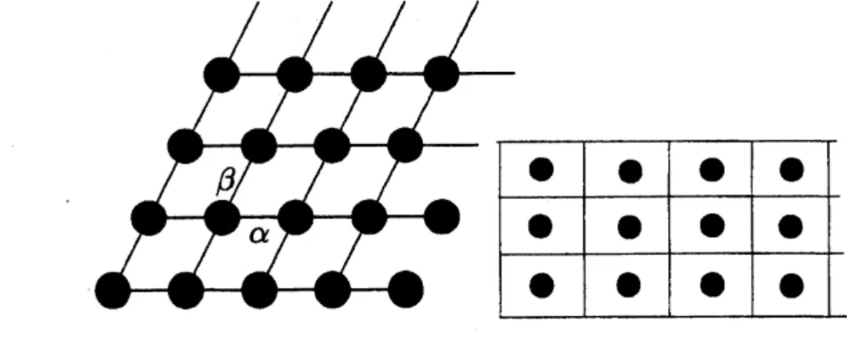
Let

$\mathrm{Y}_{\Sigma}=$

{

(_{$x_{1}$},_{$x_{2}$}); there exist $s$,$t\in(0,1)$ such that $x_{1}+ix2=s\alpha+t\beta$

}

be

a

unit of

par-allelogram. See Figure 3.

Figure 3 Periodic Circular Patterns $U_{\Sigma}$

One can show that the energy density for the triangle pattern (Figure 4) is larger

than the hexagonal pattern (Figure 2).

$\epsilon\epsilon$

We will showthat the energy density defined above achieves the minimum when I i$\mathrm{s}$

ahexagonalstructure. Thenwe willobtainthe upper bound for the$\min I_{\epsilon}$ for arbitrary

domains by hexagonal structures, making a close study ofthe

error

by

an.

Proposition 3.2 (X. Chen

&

Y. Oshita). The following statements hold:

(1) For I $=$ Za$+\mathbb{Z}\beta$, $\zeta=\beta/\alpha$, ${\rm Im}(\zeta)>0,$

$\mathcal{E}[U_{\Sigma}]=\frac{2}{c_{o}}\sqrt{\frac{2\pi(1+m)}{|\mathrm{Y}_{\Sigma}|}}+\frac{\kappa(1+m)^{2}[R(\zeta)+c_{1}(m)]|\mathrm{Y}_{\Sigma}|}{2D}$,

where

$R( \zeta)=-\frac{1}{2\pi}\log|$$\mathrm{i}$ $q^{1/12} \prod_{n=1}^{\infty}(1-q^{n})^{2}|$ , $q=e^{2\mathrm{w}}i($

and

$c_{1}(m)=\mathit{7}$ $(1+$ $\mathrm{j}$ $-\log(2\pi(1+7\mathrm{r}\mathrm{z}))$

)

(2) The minimum

_of

$\mathcal{E}[U_{\Sigma}]$ among allpossible per iodic circular patterns is

$\mathcal{E}^{*}=3(1+m)(c_{o})^{-2/3}D^{-1/3}[\pi\kappa(c_{1}(m)+R(\zeta^{*}))]^{1/3}$ , $\zeta^{*}=e^{i\pi/3}$,

which is attained when ) _{is equal to the lattice} $\mathbb{Z}\alpha^{*}+\mathbb{Z}\beta’$,

$|\mathrm{c}\mathrm{z}$’$|=|$

d’

$|=2\pi^{1/6}3^{-1/4}(1+m)^{-1/2}D^{1/3}[c_{o}\kappa(c_{1}(m)+R(\zeta^{*}))]^{-1/3}$, $\frac{\beta^{*}}{\alpha}*=\zeta^{*}$.

(3) Let $\Omega\subset \mathbb{R}^{2}$ be a bounded

domain with the smooth boundary $\partial\Omega$. Then

$\min$ $I_{\epsilon}[u]\leq|\Omega|\epsilon^{2/3}[\mathcal{E}^{*}+O(\epsilon^{1/3}|\log\epsilon|)]$, $u\in H^{1}(\Omega)$

$\mathcal{E}^{*}=3(1+m)(c_{o})^{-2/3}D^{-1/3}[\pi\kappa(c_{1}(m)+R(\zeta’))]^{1/3}$, $\zeta^{*}=e^{i\pi/3}$,

which is attained when $\Sigma$ is equal to the lattice

$\mathbb{Z}\alpha^{*}+\mathbb{Z}\beta^{*}$,

$|\alpha’|=|\beta’|=2\pi^{1/6}3^{-1/4}(1+m)^{-1/2}D^{1/3}[c_{o}\kappa(c_{1}(m)+R(\zeta^{*}))]^{-1/3}$ , $\frac{\beta^{*}}{\alpha}*=\zeta^{*}$.

(3) Let $\Omega\subset \mathbb{R}^{2}$ _$6e$ a bounded

domain with the smooth boundary $\partial\Omega$. Then

$\min_{u\in H^{1}(\Omega)}I_{\epsilon}[u]\leq|\Omega|\epsilon^{2/3}[\mathcal{E}^{*}+O(\epsilon^{1/3}|\log\epsilon|)]$ ,

as

$\epsilon$ $arrow 0.$

References

[1] G. Alberti and S. Miiller. A new approach to variational problems with multiple

scales. Comm. Pure Appl. Math., Vol. 54, pp. 761-825,

2001.

[2] X. Chen.

Generation

and propagation of interfaces in reaction-diffusion systems. Trans. Amer, _{Math. Soc, Vol. 334, pp. 877-913, 1992.}

[3] X. Chen, D. Hilhorst, and E. Logak. Asymptotic behavior of solutions of an

allen-cahn equation with a nonlocal term. Nonlinear Anal. $TMA$., Vol. 28, pp.

1283-1298, 1997.

[4] R. Choksi. Scaling laws in microphase separation of diblock copolymers. J. Non-linear Sci., Vol. 11, No. 3, pp. 223-236, 2001.

[5] $\mathrm{G}.\mathrm{B}$

.

Ermentrout, $\mathrm{S}.\mathrm{P}$

.

Hastings, and $\mathrm{W}.\mathrm{C}$. Troy. Large amplitude stationary

waves

in an excitable lateral-inhibitory medium. SIAM. J. Appl. Math., Vol. 44, No. 6, pp. 1133-1149,1984.

[6] P. C. Fife. Dynamics

_for

inter$mal$ layers and

diffusive

interfaces.

CCMS-NSF

Regional Conf. Ser. in Appl. Math. SIAM, Philadelphia, 1988.

[7] P. C. Fife and L. Hsiao. The generation and propagation of internal layers. Non-linear Analysis, Vol. 12, pp. 19-41, 1988.

[8] $\mathrm{G}.\mathrm{A}$

.

Klaasen and $\mathrm{W}.\mathrm{C}$. Troy. Stationary

wave

solutions of a system of

reaction-diffusion equations derived from the FitzHugh-Nagumo equations. Siam. J. Appl.

Math., Vol. 44, pp. 96-110, 1984.

[9] S. Miiller. Singular perturbations as a selection criterion for periodic minimizing sequences. Calc. $Var$

.

Partial

Differential

Equations, Vol. 1, No. 2, pp. 169-204,

1993.

[10] Y. Nishiura and I. Ohnishi. Some mathematical aspects of the micrO-phase sepa-ration in diblock copolymers. Phys. $D$, Vol. 84, pp. 31-39, 1995.

[11] Y. Nishiura and H. Suzuki. Noexistence of higher dimensional stable turing pat-terns in the singular limit. Siam. J. Math. Anal, Vol. 29, pp. 1087-1105, 1998.

[12] I. Ohnishi,Y. Nishiura, M. Imai, and Y. Matsushita. Analytical solutiondescribing the phase separation driven by a free energy functional containing a long-range interaction term. Chaos, Vol. 9, pp. 329-341, 1999.

[13] Y. Oshita. On stable stationary solutions and mesoscopic patterns for FitzHugh-Nagumo equations inhigher dimensions. J.

_Differential

Equations, Vol. 188, No. 1, pp. 110-134, 2003.

[14] P. Pedregal. Parametrized Measures and Variational Principles, Progress in Non-linear Partial

_Differential

Equations. Birkh\"auser, 1997.

[15] X. Ren and J. Wei. Concentrically layeredenergy equilibriaofthe didiblock

copoly-mer

problem. Func. $Jnl$

of

Applied Math., Vol. 13, pp. 479-496, 2002.

[4] R. Choksi. Scaling laws in microphase separation of diblock copolymers. J. Non-linear Sci., Vol. 11, No. 3, pp. 223-236, 2001.

[5] $\mathrm{G}.\mathrm{B}$

.

Ermentrout, $\mathrm{S}.\mathrm{P}$

.

Hastings, and $\mathrm{W}.\mathrm{C}$. Troy. Large amplitude stationary

waves

in an excitable lateral-inhibitory medium. SIAM. J. Appl. Math., Vol. 44, No. 6, pp. 1133-1149,1984.

[6] P. C. Fife. Dynamics

_for

internal layers and

_diffusive

_interfaces.

CCMS-NSF

Regional Conf. Ser. in Appl. Math. SIAM, Philadelphia, 1988.

[7] P. C. Fife and L. Hsiao. The generation and propagation of internal layers. Non-linear Analysis, Vol. 12, pp. 19-41, 1988.

[8] $\mathrm{G}.\mathrm{A}$

.

Klaasen and $\mathrm{W}.\mathrm{C}$. Troy. Stationary

wave

solutions of a system of

reaction-diffusion equations derived from the FitzHugh-Nagumo equations. Siam. J. Appl.

Math., Vol. 44, pp. 96-110, 1984.

[9] S. M\"uller. Singular perturbations as aselection criterion for periodic minimizing

sequences. Calc. $Var$

.

Partial

Differential

Equations, Vol. 1, No. 2, pp. 169-204,

1993.

[10] Y. Nishiura and I. Ohnishi. Some mathematical aspects of the micrO-phase sepa-ration in diblock copolymers. Phys. $D$, Vol. 84, pp. 31-39, 1995.

[11] Y. Nishiura and H. Suzuki. Noexistence of higher dimensional stable turing pat-terns in the singular limit. Siam. J. Math. Anal, Vol. 29, pp. 1087-1105,1998. [12] I. Ohnishi,Y. Nishiura, M. Imai, and Y. Matsushita. Analytical solutiondescribing

the phase separation driven by affee energy functional containing a long-range interaction term. Chaos, Vol. 9, pp. 329-341, 1999.

[13] Y. Oshita. On stable stationary solutions and mesoscopic patterns for FitzHugh-Nagumo equations inhigher dimensions. J.

_Differential

Equations, Vol. 188, No. 1, pp. 110-134, 2003.

[14] P. Pedregal. Parametrized Measures and Variational Principles, Progress in Non-linear Partial

_Differential

Equations. Birkh\"auser, 1997.

[15] X. Ren and J. Wei. Concentrically layeredenergy equilibriaofthe didiblock

copoly-mer

problem. Func. $Jnl$

of

Applied Math., Vol. 13, pp. 479-496, 2002.