BIRATIONAL MAPS WITH SPARSE POST-CRITICAL SETS (Complex Dynamics)

56

BIRATIONAL MAPS WITH SPARSE

POST-CRITICAL

SETS

JEFFREY DILLER

1. A FAMILY OF BIRATIONAL MAPS

Very little is knownconcerning global dynamics of holomorphic maps in

dimen-sions larger than

one.

Results that apply to large classes of maps (say polynomial

automorphisms of $\mathrm{C}^{2}$ [BLS]

or

endomorphisms of

$\mathrm{P}^{n}[\mathrm{B}\mathrm{D}]$, for example)

are

con-finedmostlytothelevel of ergodic theory, describing dynamics ‘almost everywhere’

with respect to natural invariant

measures

and currents. More detailed accounts

exist only for specific examples. The immediate purpose of this exposition is to

discuss

one

such example atlength. Alongthe way I hope to also

serve

the broader

purposes of makingtheoremsabout generalmaps

more

accessible and of indicating

$\iota$

promising places to look for further tractable examples. All of the work described

here is joint with Eric Bedford and appears in

more

complete formin the preprint

[BD2]

We will consider the

one

parameter family of maps, given in affine coordinates

by

$f(x, y)=(y \frac{x+a}{x-1},x+a-1)$

.

(1) One checks easily that $f$ is Invertible, at least away from

a

couple of ‘exceptional’

curves

along which the behavior of$f$ is either degenerate or undefined

on

$\mathrm{C}^{2}$

.

In

fact $f$ extends

as

a

so-called birational map to any complexsurface compactifying

$\mathrm{C}^{2}$

.

However,

as

I will explain now, it is particularly convenient

to regard $f$

as a

birational self-mapof $\mathrm{P}^{1}\mathrm{x}$$\mathrm{P}^{1}O$

.

Modulo linear equivalence $\sim$

,

the divisors in$\mathrm{P}^{1}\mathrm{x}$ $\mathrm{P}^{1}$

form

a

group (the Picard

group) Pic$(\mathrm{P}^{1}\mathrm{x} \mathrm{P}^{1})\cong \mathrm{Z}\mathrm{x}$ $\mathrm{Z}$ generated by

a

vertical line $V:=$ [

$x$ $=$ const] and

a

horizontal

line $H:=$ [$y$ $=$ const]. Using $f$ to pull back local defining functions

for divisors,

we

obtain

a

linear action $f^{*}$ ondivisors. This action clearly preserves

linear equivalence and

so

descends to

a

linear map $f^{*}$ : Pic$(\mathrm{P}^{1}\mathrm{x} \mathrm{P}^{1})C$

on

the

Picard

group.

From the above formula,

ones

sees

that horizontal lines pull back to vertical lines, and vertical

lines

pull

back

to hyperbolas with $\mathrm{h}\mathrm{o}\mathrm{r}\mathrm{i}\mathrm{z}\mathrm{o}\mathrm{n}\mathrm{t}\mathrm{a}\mathrm{l}/\mathrm{v}\mathrm{e}\mathrm{r}\mathrm{t}\mathrm{i}\mathrm{c}\mathrm{a}\mathrm{l}$

asymptotes. Hencewith respect to the ordered basis $(V, H)$

$f^{*}=(\begin{array}{ll}\mathrm{l} 11 0\end{array})$. (2)

In particular, thespectral radiusof$f^{*}$ is the golden ratio $(1+\sqrt{5})/2$

.

The

dynam-ical

relevance

ofthis quantity is revealed by the followingresult due essentially to

Gromov (see Dinh andSibony [DS] forthe most generalversionto date)

Date: January 29,2004

57

version 10/25/01

Theorem 1.1. Let $f$ : $X\mathrm{c}^{*}\backslash$ be

a

birational map

on

a complex projective

surface

X. Then the topological entropy $h_{to\mathrm{p}}(f)$

of

$f$

satisfies

$h_{top}(f) \leq\lim_{narrow\infty}\frac{\log||(f^{n})^{*}||}{n}$

.

In addition, Dujarciin [Duj] has recently shown that this inequality is actually an

equality for a large class of birational maps (including those in (1). So for $f$given

by (1) we have

$h_{top}(f)= \log\frac{1+\sqrt{5}}{2}$

provided that

$(f^{n})^{*}=(f")$’ forall $n\in \mathrm{N}$

.

(3)

This latter identity can fail dram atically in general, but

we

will

see

shortly that

it holds for the family (1) for all but countably many values of the parameter $a$.

Forn\^a

ss

and Sibonycall maps satisfying (3) algebraically stable.

It should perhaps be stressed that (3) is

a

property of both the map and the

choice

_of

compactification

_of

$\mathrm{C}^{2}$

. For example, if I

were

treating $f$ as a self-map of

$\mathrm{P}^{2}$, then the Picard group acted

on

by _$f^{*}$ would be one-dimensional, generated by

a generic line in $\mathrm{P}^{2}$, and

$f^{*}$ would simply double this generator. However, $(f^{2})^{*}$

would multiply by3 (checkthis!) rather than $2^{2}=4$. Thus the surface $\mathrm{P}^{1}\mathrm{x}$ $\mathrm{P}^{1}$ is

‘compatible’ with the map $f$ in

a

way that $\mathrm{P}^{2}$ is not,

To better understand the situation, let

us

reconsider things from

a

geometric

point of view. On $\mathrm{P}^{1}\mathrm{x}$ $\mathrm{P}^{1}$, the critical set

$\mathrm{C}(f)$ of $f$ is the pair of lines $\{x=$

$-a\}\cup\{x=1\}$

.

As is the

case

for

birational

maps generally, the components of

$\mathrm{C}(f)$

are

critical because they

are

exceptional : each is mapped to

a

single

$\mathrm{p}\mathrm{o}\mathrm{i}\mathrm{n}\mathrm{t}^{1}$:

$\{x=-a\}$ to $(0,$$-1)$ and $\{x=1\}$ to $(\mathrm{o}\mathrm{o}, a)$. Consequently, the inverse map

$f^{-1}(x, y)=(y-a+1, x \frac{y-a}{a+1})$

cannot be defined continuously at either image point, a fact which one can verify

directly from the formula for$f^{-1}$. Theset $I(f^{-1}).--\{(0, -1), (\infty, a)\}$ is called the

indeterminacy set of$f^{-1}$. $\mathrm{S}\mathrm{i}\mathrm{n}\dot{\mathrm{u}}\mathrm{l}\mathrm{a}\mathrm{r}$ analysis reveals that

$\mathrm{C}(f^{-1})=\{y=-1\}\cup\{y=a\}$ $I(f)=\{(-a, \infty), (1, 0)\}$

.

If

we

change

our

compactification of $\mathrm{C}^{2}$, the sets $\mathrm{C}(f^{\pm\iota})$ and $I(f^{\pm 1})$

are

all prone

to change

as

well. It turns out (in general) that (3) is equivalent to

$fnC(f)\cap f^{-m}\mathrm{C}(f)=\emptyset$ for all $n$,$m>0$ (4)

In other words $f$ satisfies (3) ifand only if‘postcritical’ orbits

$P\mathrm{C}(f):=\cup f^{n}\mathrm{C}(f)n>0$’ $P\mathrm{C}(f^{-1})\cup f^{-m}\mathrm{C}m>0$

$(f^{-1})$

avoid eachother.

Thecondition (4) has

a

deceptivelysimple appearance. For general maps, it

can

be quite difficult to verify, because it requires knowing about the full orbit of each

lWhen $V$is acurvethat meets$I(f)$,wedefine $f(V)$to be the set$f(V-\mathrm{I}(\mathrm{f})$. Inotherwords,

$f(V)$is theproper_transformof$V$andexcludes allcomponentsof$C(f^{-1})$

.

This notion of$f(V)$does

not entirely accord with that of $f_{*}V:=(f^{-1})^{*}V$: in general$f(V)\subset \mathrm{s}\mathrm{u}\mathrm{p}\mathrm{p}f_{*}V$, butthe inclusion

will be proper when $V\cap I(f)\neq\emptyset$. To take a concreteexample, we have $f(\{x=a\})=(0, 1)$,

58

version 10/25/01

component of$\mathrm{C}(f)$

.

Things

are

easier,however,for theexample at hand. Our map

$f$ has the additional virtue that it preserves ameromorphic two form:

$f^{*} \eta=f_{*}\eta=\eta:=\frac{dx\mathrm{A}dy}{y-x+1}$

.

It follows

more

or less immediately that the support of the divisor

$[\eta]=[x=\infty]+[/?=\infty]+[y=x-1]$

of$\eta$ is invariant under $f$. Direct computation with parametrizations reveals

more

specifically that $\{y=x-1\}$ is fixed and the lines at infinity

are

switchedaccording

to

$(\mathrm{x},\mathrm{x}-1)\mapsto(x+a, x+a-1)$ $(\infty, y)-\rangle(y, \infty)\mapsto(\infty,y+a-1)$

.

In particular, the point $(\infty, \infty)$ is fixed by $f$

.

Invarianceof$\eta$ also implies that critical components of$f$ mustmapinto

$\mathrm{s}\mathrm{u}\mathrm{p}\mathrm{p}[\eta]$

.

Hence $\mathrm{V}\mathrm{C}\{\mathrm{f}$) $P\mathrm{C}(f^{-1})\subset \mathrm{s}\mathrm{u}\mathrm{p}\mathrm{p}[\eta]$, and the happy consequence is that

we can

de-termine whether ornot $f$ satisfies (4) by restricting

our

attentionto the completely

tractable one dimensional dynamics of$f$

on

$\mathrm{s}\mathrm{u}\mathrm{p}\mathrm{p}[\eta]$

.

2. REAL DYNAMICS FOR NEGATIVE PARAMETERS

Though

we

could easily, in light of the preceedingdiscussion, identify all

param-eters $a$ for which (4) fails, let

us

attend only to the

case

$a<0$

.

The parameter

$a=-1$ is special, because the first coordinate of $f$ degenerates, the critical and

indeterminacy sets disappear, and the map dynamics become trivial. For all other

$a<0$, (4) holds inaparticularly robust fashion. For example $P\mathrm{C}(f)\cap\{y=x-1\}$

isjust the forward orbit of the point (-1,0). Ifwe let

$S:=$

{

($x$,x-l) : $x\leq 0$

}

be the real interval in $\{y=x-1\}$ that

stretches

from (-1,0) down and left to

$(\infty, \infty)$, then

we

see

that$f(S)\subset S$when$a<0$

.

Therefore$P\mathrm{C}(f)\cap$

{

$y=$

x-l}

$\subseteq S$.

Likewise the interval

$U:=$ $\{ (\mathrm{x}, \mathrm{x}-1) :x\geq 1\}$

stretching from $(1, 0)$ up and rightto $(\infty, \infty)$ satisfies$f^{-1}(U)\subseteq U$when $a<0$ and

therefore contains $P\mathrm{C}(f^{-1})\cap\{y=x-1\}$

.

As $U$ and $S$ are disjoint, it follows that

$VC\{f$)$\cap P\mathrm{C}(f^{-1})$ contains

no

points in $\{y=x-1\}$

.

Similar observations apply to the lines $\{x=\infty\}$ and $\{y=\infty\}$

.

When $a<0$,

each line contains disjoint, $\mathrm{f}\mathrm{o}\mathrm{r}\mathrm{w}\mathrm{a}\mathrm{r}\mathrm{d}/\mathrm{b}\mathrm{a}\mathrm{c}\mathrm{k}\mathrm{w}\mathrm{a}\mathrm{r}\mathrm{d}$ invariant, real intervals $S$ and $U$

separating$VC(f)$ from $P\mathrm{C}(f^{-1})$

,

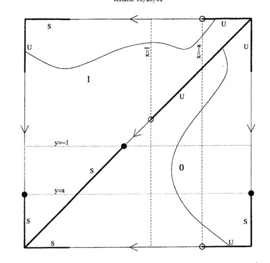
and it follows that $P\mathrm{C}(f)$ $\cap P\mathrm{C}(f^{-1})$ is empty.

Figure 1 summarizesthis state ofaffairs for $a<-1$

.

The realpointsin $\mathrm{P}^{1}\mathrm{x}$$\mathrm{P}^{1}$

form

a

torus. Removing $\mathrm{s}\mathrm{u}\mathrm{p}\mathrm{p}[\eta]$ divides the remaining real points into two open

sets, labeled 0 and 1. The boundary of each open set is exactly equal to the real

points in $\mathrm{s}\mathrm{u}\mathrm{p}\mathrm{p}[\eta]$

.

$\mathrm{S}(\mathrm{t}\mathrm{a}\mathrm{b}\mathrm{l}\mathrm{e})$ and $\mathrm{U}(\mathrm{n}\mathrm{s}\mathrm{t}\mathrm{a}\mathrm{b}\mathrm{l}\mathrm{e})$ segments in each boundary component

are

thickened for emphasis. Finally, thecritical andindeterminacysetsof$f$ and$f^{-1}$

are

included for thesake of completeness. Thepicture remainsvalid forparameter

values

$-1<a<0$

, except that the critical lines for $f$ (andfor $f^{-1}$) switch places.

Let

us

regard two stab le segments that are adjacent in the boundary of region

0 or

1

as

part of asingle larger boundary segment. In this way, the boundaries of

regions 0 and 1 may be regarded

as

‘rectangles’, eachwithopposing pairs of stable and unstable ‘sides’. This suggests that for real parameters $a$,

we

try to use the

ss

version 10/25/01

FIGURE 1. Real partition by supp7. The critical set of $f/f^{-1}$

is shown

as

$\mathrm{d}\mathrm{a}\mathrm{s}\mathrm{h}\mathrm{e}\mathrm{d}/\mathrm{d}\mathrm{o}\mathrm{t}\mathrm{t}\mathrm{e}\mathrm{d}$lines, indeterminacy set of $f/f^{-1}$

as

$\mathrm{h}\mathrm{o}\mathrm{l}\mathrm{l}o\mathrm{w}/\mathrm{s}\mathrm{o}\mathrm{l}\mathrm{i}\mathrm{d}$ circles, and sample stable

arcs as

wavy lines. The

arrows

indicate the directionofmotion of points under iterationof

$f$

.

two regions

as

a Markov partition for the dynamics of $f$

.

Let I be the space of

$\mathrm{b}\mathrm{i}$-infinite sequences $\{$0, 1$\}^{\mathrm{Z}}$ (with the product topology) and

$D:=$

{

$p\in \mathrm{R}^{2}$ : $fn(p)\not\in \mathrm{s}\mathrm{u}\mathrm{p}\mathrm{p}[\eta]$ for all $n\in \mathrm{Z}$

}

$=\mathrm{R}^{2}-\mathrm{s}\mathrm{u}\mathrm{p}\mathrm{p}[\eta]-\cup \mathrm{C}(f^{n})n\in \mathrm{Z}$

consist of those points whose orbits lie entirely in the interior of regions 0 and 1.

Define

a

map

$w$ : $Darrow\Sigma$, $p\mapsto\ldots w_{-1}w_{0}\cdot w_{1}w_{2}\ldots$ ,

where$w_{j}\in\{0, 1\}$ records the region that contains $f^{j}(p)$

.

It is nothard to

see

that $w$ is continuous. Moreover, ifa: $\Sigma \mathcal{O}$ is the shift homeomorphism

. .

.

$w_{-1}w_{\mathrm{f}1}\cdot w_{1}w_{2}$

. . .

$\mapsto\sigma$

.

.

.

$w_{-1}w_{0}w_{1}$

.

$w_{2}$

.

. .

,

then

we

clearlyhave a commutative diagram

$D$ $arrow f$ $D$

$w\downarrow\Sigma$ $arrow\sigma$

so

version 10/25/01

More importantly and muchless obviously,

we can

say

a

great deal about the fiber

of$w$

over

any point in $\Sigma$

.

Consider the following subsets of$D$

.

$D_{+}$ $=$ $\{p\in D : \lim_{narrow\infty}f^{n}p=(\infty, \infty)\}$

$D_{-}$ $=$ $\{p\in D : \lim_{narrow\infty}f^{-n}p=(\infty, \infty)\}$

$\Omega$ _$=$ $D-D_{+}-D_{-}$.

Let

us

call the coding $w(p)$ of$p\in D$

forward

alternating if

some

righthand tail

$u_{j}’ w_{j+1j+2}u)$

.

.

.

of$w(p)$hasthe form0101.

.

..

Letuscall$w(p)$ backwardalternating

if

some

lefthand tail

. . .

$w_{j-2}w_{j-1}w_{-j}$ has the analogous property. Let $\Sigma_{G}\subseteq\Sigma$

denote the (closed) subset consistingofallsequences without consecutive 1’s. The

main result of this exposition is

Theorem 2.1. Suppose that a $<0$, a $\neq-1$

.

Let p $\in D$ he any point Then

$\bullet$ $p\in D_{+}$

if

and only

if

$w(p)$ is

forutard

alter ating.

$\bullet$ $p\in D_{-}$

if

and only

if

$w(p)$ is backward alternating.

Finally, $w$ : $\Omegaarrow\Sigma$ is a homeomorphism onto those sequences in $\Sigma_{G}$ that

are

neither

_forward

nor backward alternating.

Since the dynamics of $f$

on

$\mathrm{s}\mathrm{u}\mathrm{p}\mathrm{p}[\eta]$

are

trivial, Theorem 2.1 gives a rather

pre-cise topological description of the real dynamics of $f$. I will quickly indicate two

consequences of this theorem and then discuss

some

ingredients of the proof.

Corollary 2.2. 0 consists exactly

_of

those points in D with recurrent orbits.

The entropy of

a

restricted map

never

exceeds that of the map itself,

so

onthis

generalprinciple

we

know that

$h_{top}(f : \Omega \mathrm{O})$$\leq h_{top}(f : \overline{\mathrm{R}^{2}}\langle 3)$$\leq h_{t\mathrm{o}\mathrm{p}}(f :\mathrm{P}^{1}\mathrm{x}\mathrm{P}^{1}\mathcal{O})=\frac{1+\sqrt{5}}{2}$

.

On the other hand, the shift map a restricts to

a

well-defined

homeomorphism

of $\Sigma_{G}$ whose entropy is well-known to be $\log\frac{1+\sqrt{-5}}{2}$

.

Since removing the relatively

small sets of$\mathrm{f}\mathrm{o}\mathrm{r}\mathrm{w}\mathrm{a}\mathrm{r}\mathrm{d}/\mathrm{b}\mathrm{a}\mathrm{c}\mathrm{k}\mathrm{w}\mathrm{a}\mathrm{r}\mathrm{d}$alternating codings does not alter the value of the

entropy, we can conclude that

Corollary 2.3. For all $a<0$, $a\neq-1$, the topological entropy

of

$f$

as

a real map

is $\log\frac{1+\sqrt{5}}{2}$.

The fundamental idea underlying Theorem 2.1 is that forward and backward images of real

arcs

may be studied in two different

ways:

from a

combinatorial

pointofviewbased

on

Figure 1, and from the

more

abstract perspectiveof complex

intersection theory. I discuss these points of view in order.

3. COMBINATORICS

Prom

now

onI will

assume

that$a<-1$

.

Icall

a

real

arc

‘stable’if it iscompletely

contained in

one

of the two regions in Figure 1 and it joins the two unstable

segmentsin the boundary of that region. Tojustify this definition, let

me

consider

forexample the preimage $f^{-1}(\gamma)$ of

a

stable

arc

$\gamma$ in region0. Say for specificity’s

sake that $\gamma$ joins the unstable segment in $\{y=x-1\}$ to the

unstable

segment

in $\{y=\infty\}$

.

Then $\gamma$ necessarily

crosses

both lines in $\mathrm{C}(f^{-1})$, and the preimage

$f^{-1}(\gamma)$ must therefore contain three subarcs:

one

joining the unstable segment in

$\epsilon$$\iota$

version 10/25/01

to $(1, 0)=f^{-1}\{y=a\}$_{, and}

one

_joining $(0,$ _$-1)$ to the unstable segment in _$\{x=$

$\infty\}=f^{-\mathrm{I}}\{y=\infty\}$. By checking theimages of points in $\gamma$

near

$\mathrm{s}\mathrm{u}\mathrm{p}\mathrm{p}[\eta]\cup \mathrm{C}(f^{-1})$,

one sees

that the first and third

arcs

lie in region 0, whereas the second lies in

region 1. In particular thesecond third subarcs joinopposing unstable segments in

regions 0 and 1, respectively, and are therefore themselves stable (the first subarc

is not stablesince

both

of its endpoints lie in the

same

unstable segment in region

0). Repeating this argument

proves

that the preimage $f^{-1}(\gamma)$ of

an

stable

arc

7 in

region 1 must contain

an

stable

arc

in region0. After induction we arrive at

Theorem 3.1. Let $m\geq 0$ and $w_{0}$

.

$w_{1}$

. .

.

$w_{m}$ be

a

finite

righthand sequence

of

0’s and

1

’s

without

consecutive 1’s. Let $\alpha$ be

a

stable

arc

in region _{$w_{m}$}

.

Then

$f^{-m}(\alpha)$ contains

a

stable

arc

$\gamma$ in region $w_{0}$ such that $f^{j}(\gamma)$ lies in region $w_{j}$

for

$j=0$, $\ldots$,$m$

.

Of course,

we

can

also define ’unstable’

arcs

in regions 0 and 1, and proceed in

exactly the

same

fashion to prove

Theorem 3.2. Let$n\geq 0$ and $w_{-n}\ldots$$w_{0}$

.

be

a

finite lefthand

sequence

of

0’s and

1 ’s without consecutive 1’s. Let $\beta$ be

an

unstable

arc

in region $w_{-n}$

.

Then $f^{n}(\beta)$

contains

an

unstable arc $\gamma$ in region $w_{0}$ such that $f^{-j}(\gamma)$ lies in region $w_{j}$

for

$j=0$,$\ldots,n$

.

The fact that stable and unstable boundary segments of regions 0 and 1

are

disjoint implies that any stable arc in a given region intersects any unstable arc

from the

same

region. SoTheorems

3.2

and3.1 give

us

a convenientway to produce

points withorbits coded byfinite two-sided

sequences

of any extent.

Corollary 3.3. Let $n$,$m\geq 0$ and $w_{-n}$ .

..

$u$)$0^{\cdot}w_{1}\ldots$ $w_{m}$ be any

finite

sequence

of

0’s and 1 ’s without consecutive 1 ’s. Then there is

a

point $p\in D$ such that

$c(p)=$ .

. .

$w_{-n}$

.

.

.

$w_{0}\cdot w_{1}$

. .

.

$u1_{m}$

. .

.

.

It is not quite immediate (and not quite true!) that the image $w(D)$ of the

coding map contains $\Sigma_{G}$, let alone that the assertions of Theorem 2.1 concerning

$w|\mathrm{r}\iota$

are

true. However, Corollary3.3is clearlyastepin the right direction. Further

progress

depends

on

refining the partition shown in Figure 1.

For any $n\geq 0$, every component in the critical set $\mathrm{C}(f^{n})$ maps, eventually, into

thestable portion of$\mathrm{s}\mathrm{u}\mathrm{p}\mathrm{p}[\eta]$

.

So

we

can

subdivide

our

originalpartitionusing$\mathrm{C}(f^{n})$

for any $n\in \mathrm{N}$

,

designating all the new boundary components ‘stabl\’e. Similarly,

we

can

subdivide by $\mathrm{C}(f^{-n})$, designating all inverse critical components ‘unstabl\’e.

And whileit is not strictlynecessary,

we

cantry to simplify the picturethatresults

by recombining

some

of thenew partition pieces, provided wetake

care

topreserve

invariance of $\mathrm{s}\mathrm{t}\mathrm{a}\mathrm{b}\mathrm{l}\mathrm{e}/\mathrm{u}\mathrm{n}\mathrm{s}\mathrm{t}\mathrm{a}\mathrm{b}\mathrm{l}\mathrm{e}$ boundary components. The result of this process,

obtained with

care

and hindsight, is shown in Figure 2. The original regions0 and

1 becomesmaller rectangles$R_{0}$ and$R_{1}$, andthecomplement of Rq URi decomposes

into overlapping regions labeled $R_{+}$ and $R_{-}$. Using only combinatorial arguments

like the

ones

above, the following

can

be established.

Proposition 3.4. The conclusion

_of

Corollary 3.3 holds with the regions 0 and 1

from

Figure 1 replaced by regions $R_{0}$ and $R_{1}$

from

Figure 2. Moreover,

$\bullet$ $f(R^{+})\subset R^{+}$, and any point $p\in R^{+}\cap D$ has $a$

forward

coding $w_{0}\cdot w_{1}\ldots$

that alternates and $a$

forward

orbit that tends to $(\infty, \infty)$

.

$\bullet$ $f^{-1}(R^{-})\subseteq R^{-}$, and

an

$\iota y$point$p\in R^{-}\cap D$ has

a backrnard

coding

..

.

$w_{-1}w0^{\cdot}$

82

version 10/25/01

FIGURE 2. Refinement ofthe original partition to include critical

curves.

Stable and unstable boundary segments arelabeled $‘ \mathrm{s}$’ and

‘$\mathrm{u}’$, respectively.

.

$f(R_{1})\cap R_{1}=\emptyset$

.

Togetherwith the following, somewhat technically difficult result; Corollary 3.3

and Proposition3.4 combine to imply everything in Theorem 2.1 except the

injec-tivity of$f|_{\Omega}$.

Proposition 3.5. Any point $p\in D$ such that $\lim_{narrow\infty}fn(p)=(\infty, \infty)$

(respec-tively, $1\mathrm{i}\iota \mathrm{n}_{narrow\infty}\mathrm{f}\mathrm{n}(\mathrm{p})$ $=(\infty, \infty))$ must satisfy $fn(p)\not\in R^{0}\cup R^{1}$ (respectively,

$f^{-n}(p)\not\in R^{0}\cup R^{1})$

for

arbitrarily large $n\in \mathrm{N}$

.

4. INTERSECTION THEORY

(5)

Here is a slightly

different

and less precise way to state Corollary

3.3.

Suppose

we are

given $\mathrm{i},j$ $\in\{0,1\}$,

a

stable

arc a

in region $\mathrm{i}$,

an

unstable

arc

$\beta$ in region$j$,

and $m,n\in$ N. Then

$f^{-m}(\alpha)\langle\cap f^{n}(\beta)$

must containat least

$(\begin{array}{ll}1 11 0\end{array})$ $n\mathrm{e}_{i}$

, $(\begin{array}{ll}1 11 0\end{array})$$m\mathrm{e}_{j}\rangle$

distinct points in $R_{0}\cup R_{1}$

.

Equation (5), in which $\mathrm{e}_{0},\mathrm{e}_{1}$

are

the

standard

basis

vectors for $\mathrm{R}^{2}$, simply counts the number of codings

$w_{-n}$.. .$w_{0}\cdot w_{1}$

..

.$w_{m}$ that

begin with digit $w_{-n}=\mathrm{i}$

,

end with digit $w_{m}=j$, and contain

no

consecutive

83

version 10/25/01

possibility that there might be

more

intersections than (5) provides. To obtain

control from above, I change tactics and consider only very special examples of

stable and unstable

curves.

Namely, I

suppose

that

a

is obtained by intersecting $R_{1\mathrm{J}}$ with a vertical line or

$R_{1}$ by the preimageof

a vertical

line, and that $\beta$ is obtained similarly. This turns

out notto betoo

severe

since both regions haveaproduct structuregiven by stable and unstable

curves

of this sort. The advantage to the restriction is that complex

intersection theory tells

us

exactly how manytimes

one

algebraic

curve

intersects

another and therefore gives us

an

upper bound

on

$\# f^{-m}(\alpha)\cap f^{n}(\beta)$

.

The data

needed to obtain this upper bound

are

the basis $(V, H)$for Pic$(\mathrm{P}^{1}\mathrm{x}\mathrm{P}^{1})$, thematrix

(2) for $f^{*}$ with respect to this basis, and additionally, the matrix

$(\begin{array}{ll}0 1\mathrm{l} 0\end{array})$

for the intersection form for complex

curves

in $\mathrm{P}^{1}\mathrm{x}\mathrm{P}^{1}$

.

The results take

a

bit of

interpreting because the algebraic

curves

giving the stable and unstable foliations

of $R_{1}$ also intersect $R_{0}$ is stable and unstable

arcs.

However in the end

we

obtain

an upper bound for $\# f^{-n\tau}(\alpha)\cap f^{n}(\beta)$ that matches (5) exactly in all

cases.

In

light of (2), we might have expected close agreement

even

before setting pencil

to paper, but exact agreement is not a priori obvious (at least not to me). It is

fortunate, though, because precise agreement between upper and lower bounds is

the main thing needed to complete the proofof Theorem 2.1 (i.e. of injectivity of

$f$ : $\Omegaarrow\Sigma_{G}.$)

Ratherthan go into

more

detail here, I will describe

some

further consequences

ofintersection theory for dynamics of $f$. By using Lefschetz’ theorem

on

periodic

points, it

can

be shown that

Theorem 4.1. All periodic points

_of

$f$

are

real. Indeed all except $(\infty, \infty)$ are

saddle points contained in $\Omega$, and saddle periodic points constitute a dense subset

of

$\Omega$

.

Sofar,I have mostly described the set $\Omega=D-D_{-}-D_{+}$ of points whose orbits

lie neither the forwardnorthe backward basin of $(\infty, \infty)$, but in fact the individual

complements of$\Omega_{+}:=D-D_{+}$ and $\Omega_{-}:=D-D_{-}$ yield to the

same

analysis.

Theorem 4.2. $\Omega_{+}$ is the support

of

a

geometric 1 current$\mu^{+}$. That is, there is $a$

lamination $\mathcal{L}^{+}$ in $\mathrm{P}^{1}\mathrm{x}\mathrm{P}^{1}$ - $\mathrm{s}\mathrm{u}\mathrm{p}\mathrm{p}[\eta]$ and

a

measure

$\iota/+$

on

the set $|\mathcal{L}|^{+}$

of

leaves

of

this lamination such that

$\bullet$ _{$\mu^{+}(\zeta)=\int_{\mathcal{L}+}|(\int_{L}\zeta)\nu^{+}(L)$}

for

all 1

forms

$\zeta \mathfrak{j}$

$\bullet \mathrm{s}\mathrm{u}\mathrm{p}\mathrm{p}\mathcal{L}^{+}=\Omega_{+};$

$\bullet$ Every

leaf of

$\mathcal{L}^{+}$ is

a

stable

curve

in regions 0 or 1

from

Figure 1;

$\bullet$ $\nu^{+}$ is invariant underholonomy along

$\mathcal{L}^{+}\mathrm{i}$

$\bullet f^{*}\mu^{+}=-\mu^{+}$

.

NotethatI

am

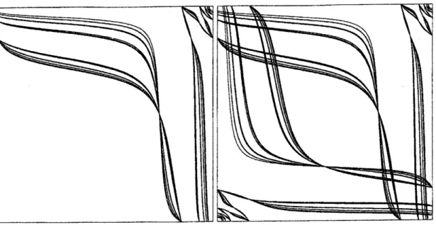
avoidingthe matterof orientationinthe first andlast items. Figure

4 shows $\mathcal{L}^{+}$ by itself and together with the corresponding lamination $\mathcal{L}^{-}$

comple-serting $D_{-}$. The

common

intersection ofthe two laminations isjust (the closure

84

version 10/25/01

FIGURE 3. Stable lamination alone (left) and with the unstable

lamination (right), for parameter $a=-2$. Note that coordinates

are

adapted to show behavior

near

infinity and that intersection

points among the leaves of$\mathcal{L}^{+}$

occur

only

on

$\mathrm{s}\mathrm{u}\mathrm{p}\mathrm{p}[\eta]$

.

5. CONCLUSION

Complex intersection theory

can

be used to study dynamics of any rational

map. Indeed the currents $\mu^{+}$ and $\mu^{-}$ have general complex analogues for any

dynamically interesting birational map, and the intersection between $\mu^{+}$ and $\mu^{-}$

can

often be understoodin at least a

measure

theoretic

sense

(see [BDIJ). What is

special to the example I have justdescribed isthe presenceof

a

goodcombinatorial

structure. In my view, there

are

two key features of the example from which the

combinatorics proceed. First of all, the post-critical orbits $P\mathrm{C}(f)$ and $P\mathrm{C}(f^{-1})$

lie in invariant

curves

and

are

therefore very easy to understand. Second, rather

than being interlaced in

some

complicated fashion, the sets $VC(f)$ and $P\mathrm{C}(f^{-1})$

are

easily separated by dividing each real invariant

curve

into

a

pair of intervals.

Some of the other aspects ofthe example, such as the perfect agreement between

intersection theory and combinatorics, remain mysterious to me, _{In aforthcoming}

paper, Bedford and I will describe another family of birational maps whose real

dynamics

can

be analyzed in a similar fashion. It does not

seem

too hard to come

by further families of maps with “sparse postcriticai sets”

so

it is interesting to

wonder how far the analysis described here

can

be extended.

REFERENCES

[BD1] Eric Bedford andJeffreyDiller. Energyand invariantmeasurefor birationalmaps, preprint.

[BD2] Eric Bedford and Jeffrey Diller. A family of plane birational maps with real dynamics

conjugate tothe Fibonaccisubshift. preprint.

[BLS] Eric Bedford, MikhailLyubich, and John Smttlie. Polynomial diffeomorphisms of$\mathrm{C}^{2}$. IV.

The measure _ofmaximalentropy and laminar cu rents. Invent. Math. 112(1993),77-125.

[BD] Jean-Yves Briend and Julien Duval. Deux caractiruations de la mesure d’iquilibre d’un

85

version 10/25/01

[DF] J. Diller and C. Favre. Dynamics of bimeromorphic maps _{of surfaces.} Amer. J. Math.

123(2001), 1135-1169.

[DS] $\mathrm{T}\mathrm{i}\mathrm{e}\mathrm{n}\sim \mathrm{C}\mathrm{u}\mathrm{o}\mathrm{n}\mathrm{g}$ Dinh and NessimSibony. Unebornesuperieurepour FentroPie. preprint.

[Duj] R. Dujardin. Laminarcurrents andentropy propertiesof surfacebirational maps,preprint. DEPARThlENTOF MATHEMATICS, UNIVERSITY OFNOTRE Dams. NOTRE DAM4E, IN 46656