LARGE DATA INCOMPRESSIBLE NONSTATIONARY FLOWS IN CYLINDRICAL DOMAINS (Mathematical Analysis of Viscous Incompressible Fluid)

全文

(1)65. 数理解析研究所講究録第2009巻 2016年 65-83. LARGE DATA INCOMPRESSIBLE NONSTATIONARY FLOWS IN CYLINDRICAL DOMAINS JOANNA RENCLAWOWICZ. ABSTRACT. We discuss the existence of solutions to the. large data incompressible non‐ cylindrical domain. The motion of the fluid is modeled using the Navier‐Stokes system with the slip boundary conditions and prescribed inflow and out‐ stationary flows. in. a. flow functions.. Key words: Navier‐Stokes equations, motions in cylindrical domains, boundary slip conditions, global existence of regular solutions, large data. MSC 2000: 35\mathrm{Q}35, 76\mathrm{D}03, 76\mathrm{D}05. 1. INTRODUCTION. problem examined in papers [\mathrm{R}\mathrm{Z}1]-[\mathrm{R}\mathrm{Z}7] related to the nonstationary, incompressible cylindrical domain. The results obtained in these papers will be the start point for further analysis of inflow‐outflow problems and next, flows around The motion is modeled with Navier‐Stokes system some obstacle, with large velocities. of equations, with slip boundary condition. The main goal is to obtain the existence result for the inflow‐outflow problem with arbitrarily large flux, where the initial velo.city does not change to much along the axis of cylinder and the inflow does not change much along directions perpendicular to this axis either with respect to time. The inflow‐outflow problem is the subject in papers [RZ4], [RZ5], [RZ6] and also [\mathrm{R}\mathrm{Z}7]- for the reverse Y‐ shaped domain. In the paper [RZ1] we consider the problem with no inflow and in [RZ2] and [RZ3] we examine an auxiliary Poisson equation in order to obtain the weighted estimates in L_{2} and L_{p} Sobolev weighted spaces, crucial for other results. Introducing some large data, like the inflow, is a diffcult question to establish global existence of regular solutions. Regularity of solutions for Navier‐Stokes equations, even with no flux, requires some smallness conditions. We underline, that our restrictions admit much more general class of solutions than, for example, in [Kl, K2, Zl, Z3] because in these papers the flux must converge to zero suffciently fast or there is no flux. Many results of this type were proved assuming smallness of initial velocity, some restrictions on domain (so called thin domain, $\Omega$=$\Omega$'\times(0, $\epsilon$), $\Omega$'\in \mathbb{R}^{2} with small $\epsilon$ ) or special We present the. ,. motion in. structure of solutions. here. (so that. the solution is close to 2‐dimensional. examples [M1], where. the existence for. solution).. We mention. large data is obtained under some geometrical constraints for 2\mathrm{d} model in steady and evolutionary case; [M2], where steady Navier‐Stokes equations in pipe‐like domain are investigated and existence is shown for a class of cylindrical symmetric solutions and [Z4], where the problem of nonstationary as some. Institute of. Mathematics, Polish Academy of Sciences, leading to these results has received funding from the People Programme (Marie Curie Actions) of the European Unions Seventh Framework Programme FP7/2007‐2013/ under REA grant agreement no 319012 and from the Funds for International Co‐operation under Polish Ministry of Science and Higher Education grant agreement no 2853/7.\mathrm{P}\mathrm{R}/2013/2. The research.

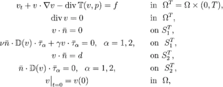
(2) 66. axially symmetric domain is examined and the result concerns the existence for axially symmetric solutions and the inflow and outflow sufficiently close to homogeneous flux. In our results there is no restrictions on magnitude of flux, moreover, in the proof of the existence of global regular solutions we admit arbitrarily large L_{2} norm of initial velocity. However, our data could not be arbitrary: if we were able to take any data then the regularity problem for the weak solutions to the Navier‐Stokes would be solved. We assume smallness of derivatives along the axis of cylinder for inflow function and initial velocity. Let us formulate the system of Navier‐Stokes equations describing the motion in papers flow in. solutions close to. [\mathrm{R}\mathrm{Z}4]-[\mathrm{R}\mathrm{Z}6]. v_{t}+v\cdot\nabla v-\mathrm{d}\mathrm{i}\mathrm{v}\mathbb{T}(v,p)=f. in. \mathrm{d}\mathrm{i}\mathrm{v}v=0. in. v\cdot\overline{n}=0. on. $\nu$\overline{n}\cdot \mathbb{D}(v)\cdot\overline{ $\tau$}_{ $\alpha$}+ $\gamma$ v\cdot\overline{ $\tau$}_{ $\alpha$}=0,. (1.1). $\alpha$=1 ,. 2,. on. v\cdot\overline{n}=d. \overline{n}\cdot \mathbb{D}(v)\cdot\overline{ $\tau$}_{ $\alpha$}=0,. on. $\alpha$=1 ,. 2,. on. v|_{t=0}=v(0) where $\Omega$\subset \mathbb{R}^{3} is. time,. v. is the. in. $\Omega$^{T}= $\Omega$\times(0, T). ,. $\Omega$^{T},. S_{1}^{T}, S_{1}^{T}, S_{2}^{T}, S_{2}^{T}, $\Omega$,. cylindrical domain (Figure 1), S=\partial $\Omega$, T<\infty is the existence velocity of the fluid motion with v(x, t)=(v_{1}(x, t), v_{2}(x, t), v_{3}(x, t))\in \mathbb{R}^{3},. p=p(x, t)\in \mathbb{R}^{1}. a. denotes the pressure,. f=f(x, t)=(f_{1}(x, t), f_{2}(x, t), f_{3}(x, t))\in \mathbb{R}^{3}. —the. field, x=(x_{1}, x_{2}, x_{3}) are the Cartesian coordinates, \overline{n} is the unit outward vector normal to the boundary S and \overline{ $\tau$}_{ $\alpha$}, $\alpha$=1 2, are tangent vectors to S and the dot denotes the scalar product in \mathbb{R}^{3}. \mathbb{T}(v,p) is the stress tensor of the form external force. .. ,. \mathrm{T}(v,p)= $\nu$ \mathbb{D}(v)-p\mathrm{I}, where. slip. $\nu$. is the constant. coefficient and. \mathbb{D}(v). viscosity. coefficient and I is the unit matrix.. Next, $\gamma$>0. is the. denotes the dilatation tensor of the form. \mathbb{D}(v)=\{v_{i,x_{j}}+v_{j,x_{i}}\}_{i,j=1,2,3}. In paper. boundary,. [RZ1]. so. we. consider the. boundary. conditions. problem (1.1) on. S. with. no. inflow and. no. friction. are zero:. v\cdot\overline{n}=0. \overline{n}\cdot \mathbb{T}(v,p)\cdot\overline{ $\tau$}_{ $\alpha$}=0,. $\alpha$=1 ,. 2,. on. S^{T},. on. S^{T}.. X3. FIGURE 1. Domain $\Omega$.. on. the.

(3) 67. $\Omega$\subset \mathbb{R}^{3} as presented on the picture is a straight cylinder parallel to the X3 arbitrary cross section. We denote the boundary of $\Omega$ by S and set S=S_{1}\cup S_{2} where S_{1} is parallel to the axis X3 and S_{2} is perpendicular to X3. Consequently, Domain. axis with. S_{1} = \{x\in \mathbb{R}^{3} : $\varphi$_{0}(x_{1}, x_{2})=c_{0}, -a<x_{3}<a\}, S_{2}(-a) = \{x\in \mathbb{R}^{3}:$\varphi$_{0}(x_{1}, x_{2})<c_{0}, x_{3}=-a\}, S_{2}(a) = \{x\in \mathbb{R}^{3}:$\varphi$_{0}(x_{1}, x_{2})<c_{0}, x_{3}=a\} $\varphi$_{0}(x_{1}, x_{2})=c_{0}. where a, c_{0} are positive given numbers and closed curve in the plane x_{3}= const. To define inflow and outflow. (d_{1}, d_{2}). with. we. specify boundary. describes. condition. where. d_{i}\geq 0, i=1. ,. 2.. condition. d_{1} =-v\cdot\overline{n}|_{S_{2}(-a)} d_{2} =v\cdot\overline{n}|_{S_{2}(a)} Using (1.1)_{2,3} and (1.2) we conclude. where $\Phi$ is the flux.. analysis that leads. to. our. on. (1.1)4 introducing. T). ,. paper. [RZ4],. [RZ1].. Regular. solutions. times T , paper. on. íntervals. [RZ6].. Controling initial data on global ones, paper [RZ6]. In Sections. 2‐5,. we. focus. on. (kT, (k+1)T). intervals. ,. [RZ5]. k\in \mathbb{N} , with estimate \mathcal{A}_{k} for. (kT, (k+1)T). and. based. with constant \mathcal{A} for. times T , paper [RZ5] and paper [RZ1] for the problem with no inflow. Existence of regular solutions on interval (0, T) for large data, paper paper. d=. following compatibility. (0, T). interval. estimates from papers [RZ2] and [RZ3]. estimates on regular solutions on interval (0,. weighted. A priori. smooth. existence result:. global. Existence of weak solutions with estimate A on. sufficiently. $\Phi$\displaystyle \equiv\int_{S_{2}(-a)}d_{1}dS_{2}=\int_{S_{2}(a)}d_{2}dS_{2},. (1.2) Plan of. the. a. prolongation. large and. large. of solutions to. these issues.. 2. WEAK SOLUTIONS AND WEIGHTED ESTIMATES. In order to formulate the weak solutions existence theorem. for the. We. study. we. define. a. space natural. of weak solutions to the Navier‐Stokes equations:. V_{2}^{0}($\Omega$^{T})=\displaystyle\{u:|u|_{V_{2}^{0}($\Omega$^{T}) \equiv\mathrm{e}\mathrm{s}\mathrm{s}\sup_{)}|u|_{L_{2}($\Omega$)}+t\in(0T)(\int_{0}^{T}|\nablau|_{L_{2}($\Omega$)}^{2}dt)^{\frac{1}{2} <\infty\}. use as. well. Lebesque. and Sobolev spaces:. isotropic and anisotropic Lebesgue. spaces:. L_{p}(Q) , Q\in\{$\Omega$^{T}, S^{T}, $\Omega$, S\}, p\in[1, \infty], L_{q}(0, T;L_{p}(Q)) , Q\in\{ $\Omega$, S\}, p, q\in[1, \infty] ; Sobolev spaces. W_{q}^{s}(Q) , Q\in\{ $\Omega$, S\}, s, q\in[1, \infty). ,.

(4) 68. anisotropic Sobolev. spaces:. W_{q}^{s,s/2}(Q^{T}) , Q\in\{ $\Omega$, S\}, s=2m, m\in \mathbb{N}, q\in[1, \infty) with the. ,. norm. \displayst le\Vertu\Vert_{W_{q}^{s,$\epsilon$/2}(Q^{T})=(_{|$\alpha$|}\sum_{+2a\leqs}\int_{Q^{T}|D_{x}^{$\alpha$}\partial_{t}^a}u|^{q}dx t)^{\frac{1}q}. where. D_{x}^{ $\alpha$}=\partial_{x_{1} ^{$\alpha$_{1} \partial_{x_{2} ^{$\alpha$_{2} \partial_{x_{3} ^{$\alpha$_{3} , | $\alpha$|=$\alpha$_{1}+$\alpha$_{2}+$\alpha$_{3}, a, $\alpha$_{i}\in \mathbb{Z}_{+}\cup\{0\}. In the. special. q=2,. case. H^{s}(Q)=W_{2}^{s}(Q) , Q\in\{ $\Omega$, S\}, s\in \mathbb{Z}_{+}\cup\{0\}, with the. Obviously, since for this. inflow. we. norm. we. \displayst le\Vertu\Vert_{H^{s}(Q)}=(\sum_{|$\alpha$|\leqs}\int_{Q}|D_{x}^{$\alpha$}u|^{2}dx)^{\frac{1}2}. well the definition of weak solution to the system (1.1), however, have to introduce some auxiliary functions in order to homogenize the. need. as. boundary condition,. going. we are. present the corresponding construction in the. to. next section.. Theorem 1. Assume the. compatibility. condition. (1.2).. Assume that. v(0)\in L_{2}( $\Omega$);f\in. L_{2}(0, T;L_{6/5}( $\Omega$));d_{i}\displaystyle \in L_{\infty}(0, T;W_{p}^{s-1/p}(S_{2}))\cap L_{2}(0, T;W_{2}^{1/2}(S_{2}));\frac{3}{p}+\frac{1}{3}\leq s, p>3 weak solution p=3, s>\displaystyle \frac{4}{3} ; and d_{i,t}\in L_{2}(0, T;W_{6/5}^{1/6}(S_{2})) i=1 2. Then there exists ,. problem (1.1). to. such that. is. v. weakly. a. ,. continuous with. converges to v_{0} as t\rightarrow 0 strongly in L_{2}(0, T;L_{2}(S_{1})) , $\alpha$=1 , 2, and v satisfies,. v. L^{2}( $\Omega$) for. all. or. respect. Moreover,. norm.. t\leq T. L^{2}( $\Omega$) v\in V_{2}^{0}($\Omega$^{T}). to t in. norm ,. v. and. v\cdot\overline{ $\tau$}_{ $\alpha$}\in. \displayst le\Vertv\Vert_{V_{2}^{0}($\Omega$^{t})^{2}+$\gam a$\sum_{$\alpha$=1}^{2}\int_{0}^{t}\Vertv\cdot\overline{$\tau$}_{$\alpha$}\Vert_{L_{2}(S_{1})^{2}\leq2\Vertf\Vert_{L_{2}(;6}^{2}0,tL_{5}($\Omega$). (2.1). + $\varphi$(\displaystyle \sup_{ $\tau$\leq t}\Vert d\Vert_{W_{3}^{s-\frac{1}{\mathrm{p} }(S_{2})})(61+\Vert v(0)\Vert_{L_{2}( $\Omega$)}^{2}\equiv A^{2}. where $\varphi$ is. a. nonlinear. positive increasing function.. To show the existence purpose,. we. To this. theorem,. we. need to obtain. an. energy. type estimate, and for this. boundary condition (1.1)5 homogeneous. functions corresponding to the inflow and outflow so. have to make the Dirichlet. end,. we. extend the. that. \tilde{d}_{i}|_{S_{2}(a_{ $\iota$})}=d_{i}, i=1, 2, a_{1}=-a, a_{2}=a We. use. the. Hopf. construction. troduce the function $\eta$. (see. papers of. Hopf [H1]. and. Ladyshenskaya [L]). :. $\eta($\sigma$; \epsilon$, \rho$)=\left{\begin{ar y}{l 1,0\leq$\sigma$\leq$\rho$e^{-1/$\epsilon$}\equivr,\ -$\epsilon$\l frac{$\sigma$}{ \rho$},r<$\sigma$\leq$\rho$,\ 0,$\rho$< \sigma$<\infty. \end{ar y}\right.. and in‐.

(5) 69. We define. (locally). functions $\eta$_{i}. on. the. $\eta$_{i}= $\eta$($\sigma$_{i}; $\epsilon$, $\rho$) , i=1, 2 where $\sigma$_{i} denote local coordinates defined. small. on a. $\Omega$ ). (inside. of S_{2}. neighborhood. by setting:. ,. neighborhood. S_{2}(a_{i}). of. :. $\sigma$_{1}=a+x_{3}, $\sigma$_{2}=a-x_{3} and. we. set. $\alpha$=\displayst le\sum_{i=1}^{2}\tilde{d}_{i}$\eta$_{i},. b = $\alpha$\overline{e}_{3}, \overline{e}_{3}=(0,0,1). .. We set. u=v-b.. Therefore,. Now. we. notice that the. not ideal. as. the. new. \mathrm{d}\mathrm{i}\mathrm{v}u. =. u\cdot\overline{n}. =. boundary. -\mathrm{d}\mathrm{i}\mathrm{v}b=-$\alpha$_{x_{3} 0. $\Omega$,. S.. on. condition for. variable: it is not. in. u. divergence. homogeneous, but the function u is us rewrite the compatibility. is. free. Let. condition. \displaystyle \int_{ $\Omega$}$\alpha$_{x_{3} dx=-\int_{S_{2}(-a)} $\alpha$|_{x_{3}=-a}dS_{2}+\int_{S_{2}(a)} $\alpha$|_{x_{3}=a}dS_{2}=0. We need to correct the function. \triangle $\varphi$. (2.2). \overline{n}\cdot\nabla $\varphi$. \displayst le\int_{$\Omega$} \varphi$dx Next,. we. define $\varphi$. as a. =. -\mathrm{d}\mathrm{i}\mathrm{v}b. in. =. 0. =. O.. u , so we. on. solution to the Neumann. problem. $\Omega$,. S,. set. w=u-\nabla $\varphi$=v-(b+\nabla $\varphi$)\equiv v- $\delta$. Consequently, (w,p). is. a. solution to the. following problem:. w_{t}+w\cdot\nabla w+w\cdot\nabla $\delta$+ $\delta$\cdot\nabla w-\mathrm{d}\mathrm{i}\mathrm{v}\mathbb{T}(w,p) =f-$\delta$_{t}- $\delta$\cdot\nabla $\delta$+ $\nu$ \mathrm{d}\mathrm{i}\mathrm{v}\mathbb{D}( $\delta$)\equiv F( $\delta$, t). in. \mathrm{d}\mathrm{i}\mathrm{v}w=0. in. w\cdot\overline{n}=0. (2.3). on. $\nu$\overline{n}\cdot \mathb {D}(w)\cdot\overline{ $\tau$}_{ $\alpha$}+ $\gamma$ w\cdot\overline{ $\tau$}_{ $\alpha$} =- $\nu$\overline{n}\cdot \mathbb{D}( $\delta$)\cdot\overline{ $\tau$}_{ $\alpha$}- $\gamma \delta$\cdot\overline{ $\tau$}_{ $\alpha$}\equiv B_{1 $\alpha$}( $\delta$) $\alpha$=1 2, \overline{n}\cdot \mathbb{D}(w)\cdot\overline{ $\tau$}_{ $\alpha$}=-\overline{n}\cdot \mathbb{D}( $\delta$)\cdot\overline{ $\tau$}_{ $\alpha$}\equiv B_{2 $\alpha$}( $\delta$) $\alpha$=1 2, ,. ,. ,. on. ,. on. w|_{t=0}=v(0)- $\delta$(0)=w(0) where \mathrm{d}\mathrm{i}\mathrm{v} $\delta$= O. Since Dirichlet. divergence free,. we can. boundary. conditions for. define weak solutions to the. w. in are. $\Omega$^{T}, $\Omega$^{T}, S^{T},. S_{1}^{T}, S_{2}^{T}, $\Omega$,. homogeneous and. problem (2.3). w. is.

(6) 70. Definition 1. We call. w. a. weak solution to. problem (2.3) if for. any. sufficiently. smooth. such that. function $\psi$. \mathrm{d}\mathrm{i}\mathrm{v} $\psi$|_{ $\Omega$}=0, $\psi$\cdot\overline{n}|_{S}=0 the. integral identity. \displaystyle \int_{$\Omega$^{\mathrm{T} w_{t}\cdot $\psi$ dxdt+\int_{$\Omega$^{T} H(w)\cdot $\psi$ dxdt+ $\nu$\int_{$\Omega$^{T} \mathb {D}(v)\cdot \mathb {D}( $\psi$)dxdt. +$\gam a$\displayst le\sum_{$\alpha$=1}^{2}\int_{S 1}^{T}w\cdot\ verline{$\tau$}_{$\alpha$} \psi$\cdot\ verline{$\tau$}_{$\alpha$}dS_{1}dt-\sum_{$\alpha,\ sigma$=1}^{2}\int_{S $\sigma$}^{T}B_{$\sigma\ lpha$} \psi$\cdot\ verline{$\tau$}_{$\alpha$}dS_{$\sigma$}dt=\int_{$\Omega$^{T}F\cdot$\psi$dx t. holds, where. H(w)=w\cdot\nabla w+w\cdot\nabla $\delta$+ $\delta$\cdot\nabla w. In order to obtain the energy estimate we use $\psi$=w multiply the first equation in (2.3) by $\psi$ , integrate by parts. as on. a. test function:. $\Omega$ and. apply. thus,. we. the definition. of F therefore ,. \displaystyle \frac{1}{2}\frac{d}{dt}\Vert w\Vert_{L_{2}( $\Omega$)}^{2}+\int_{ $\Omega$}(w\cdot\nabla $\delta$\cdot w+ $\delta$\cdot\nabla w\cdot w)dx-\int_{ $\Omega$}\mathrm{d}\mathrm{i}\mathrm{v}\mathb {T}(w+ $\delta$,p) =\displaystyle \int_{ $\Omega$}(f-$\delta$_{t}- $\delta$\cdot\nabla $\delta$) We. use. the. boundary conditions on S_{1} equality and obtain:. and. S_{2}. (1.1). in. and. apply the. .. .. wdx wdx.. Korn. inequality. to. reformulate this. \displayst le\frac{1}2\frac{d} t}\Vertw\Vert_{L 2}($\Omega$)}^{2}+$\nu$\Vertw\Vert_{H^{1}($\Omega$)}^{2}+$\gam a$\sum_{$\alpha$=1}^{2}\Vertw\cdot\overline{$\tau$}_{$\alpha$}\Vert_{L 2}(S_{1})^{2} \displaystyle\leq-\int_{$\Omega$}(w\cdot\nabla$\delta$\cdotw+$\delta$\cdot\nablaw\cdotw)dx+c\sum_{$\alpha$=1}^{2}\Vert$\delta$\cdot\overline{$\tau$}_{$\alpha$}\Vert_{L_{2}(S_{1})^{2}. +c\displaystyle \Vert \mathb {D}( $\delta$)\Vert_{L_{2}( $\Omega$)}^{2}+\int_{ $\Omega$}(f-$\delta$_{t}- $\delta$\cdot\nabla $\delta$)wdx.. The most difficult terms some. example. and focus. \displayst le\int_{$\Omega$} \delta$\cdot\nabl w We. yields. can. estimate. some. .. are. on. wdx. those caused. the. by nonlinearity w\cdot\nabla w. .. Let. us. look closer at. integral. \displaystyle\int_{$\Omega$}(b+\nabla$\varphi$)\cdot\nablaw = \displaystyle \int_{ $\Omega$}b\cdot\nabla w\cdot wdx+\int_{ $\Omega$}\nabla $\varphi$\cdot\nabla w. wdx=I_{1}+I_{2}. =. .. wdx. I_{1} using the Hölder inequality and,. moreover, the local. support of b. smallness:. |I_{1}|\leq\Vert\nabla w\Vert_{L_{2}( $\Omega$)}\Vert w\Vert_{L_{6}( $\Omega$)}\Vert b\Vert_{L_{3}( $\Omega$)}\leq c\Vert w\Vert_{H^{1}( $\Omega$)}^{2}\Vert b\Vert_{L_{3}(\overline{S}_{2}( $\rho$))}. \leq c$\rho$^{1/6}\Vert w\Vert_{H^{1}( $\Omega$)}^{2}\Vert b\Vert_{L_{6}(\overline{S}_{2}( $\rho$) }\leq c$\rho$^{1/6}\Vert w\Vert_{H^{1}( $\Omega$)}^{2}\Vert $\delta$\Vert_{L_{6}( $\Omega$)} \leq c$\rho$^{1/6}\Vert w\Vert_{H^{1}( $\Omega$)}^{2}\Vert\tilde{d}\Vert_{H^{1}( $\Omega$)} where. \overline{S}_{2}( $\rho$)=\{x\in $\Omega$ : x_{3}\in(-a, -a+ $\rho$)\cup(a- $\rho$, a)\}=\overline{S}_{2}( $\rho$, a_{1})\cup\overline{S}_{2}( $\rho$, a_{2}). ..

(7) 71. We estimate I_{2}. as. follows:. |I_{2}|=\displaystyle\int_{$\Omega$}\nabla$\varphi$\cdot\nablaw\cdotwdx|\leq\Vert\nabla$\varphi$\Vert_{L_{3}($\Omega$)}\Vertw\Vert_{L_{6}($\Omega$)}\Vert\nablaw\Vert_{L_{2}($\Omega$)} To extract in. some. small parameter. weighted Sobolev. the result of. we use. [RZ3]. on. the Poisson. problem (2.2). spaces. \Vert\nabla $\varphi$\Vert_{L_{3}( $\Omega$)} \leq c\Vert\nabla $\varphi$\Vert_{L_{3,-$\mu$'}( $\Omega$)}\leq c\Vert\nabla_{x_{3} \nabla $\varphi$\Vert_{L_{3,1-$\mu$'}( $\Omega$)}\leq c\Vert $\varphi$\Vert_{L_{3,1-$\mu$'}^{2}( $\Omega$)} \leq c\Vert \mathrm{d}\mathrm{i}\mathrm{v}b\Vert_{L_{3,1- $\mu$},( $\Omega$)} where. we. denote. |u\displayst le\Vert_{L p,$\mu$}^{k}($\Omega$)}=(\sum_{|$\alpha$|=k}\int|D_{x}^{$\alpha$}u|_{\min_{\mathrm{i}=1,2}^{p}|(\mathrm{d}\mathrm{i}\mathrm{s}\mathrm{t}(x,S_{2}(a_{i})|^{p$\mu$}dx)^{1/p},. $\mu$\in \mathbb{R},p\in(1, \infty). .. approach we use the explicit form of solutions, and for apply regularizer technique. In L_{p}, p>2 weighted spaces we need the result for p=3 (since ), we introduce some auxiliary problem and more subtle techniques to compare norms of solutions even for different weights. Note as well, that weight of the form x_{3}^{ $\mu$},p\in(1, \infty) is not the Muckenhaupt weight so the results of Coifmann‐Feffermann [CF] can not be applied. Let. us. emphasize,. that in L_{2}. the existence result. the. we. To estimate the last norm,. we. choose. \displaystyle \frac{2}{3}\leq 1-$\mu$'\leq 1. .. With. $\mu$=1-$\mu$'. we. have. c\displayst le\Vert\mathrm{d}\mathrm{i}\mathrm{v}b\Vert_{L 3,$\mu$}($\Omega$)}\leqc$\epsilon$(\sum_{i=1}^{2}\int_{\overline{S}_{2}(a_{$\iota$})|\tilde{d}_{i|^{3}\frac{$\sigma$_{i}^3$\mu$}{$\sigma$_{i}^3}dx)^{1/3}+(\sum_{i=1}^{2}\int_{\overline{S}_{2}(a_{x})|\tilde{d}_{i,x_{3}|^{3}|$\rho$(x)|^{3$\mu$}dx)^{1/3}. \displaystyle\leqc\sum_{i=1}^{2}$\epsilon$(\sup_{x_{3}\int_{S_{2}(a_{\mathrm{t})|\tilde{d}_{i}|^{3}dx'\int_{r}^{$\rho$}\frac{$\sigma$_{i}^{3$\mu$}{$\sigma$_{i}^{3}d$\sigma$_{i})^{1/3}+\sum_{i=1}^{2}(_{x}\sup_{3}\int_{S_{2}(a_{\mathrm{z})|\tilde{d}_{i,x_{3}|^{3}dx'\int_{0}^{$\rho$} \sigma$_{i}^{3$\mu$}d$\sigma$_{i})^{1/3}. \displaystyle \leq c $\epsilon \rho$^{ $\mu$-2/3}\sup_{x_{3} \Vert\tilde{d}\Vert_{L_{3}(S_{2}),3}+c$\rho$^{ $\mu$+1/3}\sup_{x_{3} \Vert\tilde{d}_{x}\Vert_{L_{3}(S_{2}). where. $\sigma$_{i}=\mathrm{d}\mathrm{i}\mathrm{s}\mathrm{t}\{S_{2} (ai), x\}, x\in S_{2}(a_{i}, $\rho$). since for. $\mu$=\displaystyle \frac{2}{3}. the r.h. \mathrm{s}. .. .. We note that the last bound holds for. takes the form. $\mu$>\displaystyle \frac{2}{3}. c\displaystyle \sup_{x_{3}}L_{3(s_{2}),3}, which cannot be made small for. large \tilde{d} Then, .. |I_{2}|\displaystyle \leq c[ $\epsilon \rho$^{ $\mu$-2/3}\sup_{x_{3} \Vert\tilde{d}\Vert_{L_{3}(S_{2}) +$\rho$^{ $\mu$+1/3}\sup_{x_{3} \Vert\tilde{d}_{x_{3} \Vert_{L_{3}(S_{2}) ]\Vert w\Vert_{H^{1}( $\Omega$)}^{2}. Let. us. notice, that in order to estimate \displaystyle \sup_{x_{3} \Vert\tilde{d}\Vert_{L_{3}(S_{2})} and \displaystyle \sup_{x}3\Vert\tilde{d}_{x_{3} \Vert_{L_{3}(S_{2})} by some W_{p}^{s} apply the Sobolev anisotropic imbedding (see [BIN], Ch.3, Section 10) which. norm we. reads. 2. 2. (\displaystyle \frac{1}{p}-\frac{1}{3})\frac{1}{s}+\frac{1}{p}\cdot\frac{1}{s}+\frac{1}{s}\leq 1 (\displaystyle \frac{1}{p}-\frac{1}{3})\frac{1}{s}+\frac{1}{p}\cdot\frac{1}{s}+\frac{1}{s}<1. for. p>3,. for. p=3..

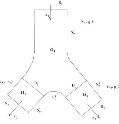
(8) 72. Thus,. find that p,. we. s. satisfy. \displaystyle\frac{3}{p}+\frac{1}{3}\leqs,. We deal with other terms in the. Sobolev. inequality,. imbedding. p>3. p=3,. or. s>\displaystyle\frac{4}{3}.. and. integral inequality. Korn. apply. inequality, Schwartz. to obtain. \displayst le\frac{1}2\frac{d} t}\Vertw\Vert_{L 2}($\Omega$)}^{2}+$\nu$\Vertw\Vert_{H^{1}($\Omega$)}^{2}+$\gam a$\sum_{$\alpha$=1}^{2}\Vertw\cdot\ verline{$\tau$}_{$\alpha$}\Vert_{L 2}(S_{1})^{2}. \leq$\varphi$_{1}( $\rho$, $\epsilon$, $\mu$, \Vert\tilde{d}\Vert_{W_{p^{S} ( $\Omega$)} \Vert w\Vert_{H^{1}( $\Omega$)}^{2}+\Vert f\Vert_{L_{6/5}( $\Omega$)}^{2}+$\varphi$_{2}(\Vert\tilde{d}\Vert_{W_{p}^{s}( $\Omega$)} (\Vert\tilde{d}\Vert_{W_{2}^{1}( $\Omega$)}^{2}+\Vert\tilde{d}_{t}\Vert_{W_{6/5}^{1}( $\Omega$)}^{2}). where $\varphi$_{i}, i=1 , 2 is a nonlinear positive increasing function and $\varphi$_{1} is small for small values of $\epsilon$, $\rho$, $\mu$ Thus, we can choose parameters $\rho$, $\epsilon$ in dependence on $\nu$ and. $\mu$>\displaystyle \frac{2}{3},. .. \Vert\tilde{d}\Vert_{W_{p}^{s}( $\Omega$)}. so. that. $\varphi$_{1}($\rho$, $\epsilon$, $\mu$,\displaystyle\Vert\ ilde{d}\Vert_{W_{p}^{s}($\Omega$)} \leq\frac{$\nu$}{2}.. Therefore,. consume the term. we can. $\varphi$_{1}\Vert w\Vert_{H^{1}( $\Omega$)}^{2}. by $\nu$\Vert w\Vert_{H^{1}( $\Omega$)}^{2} on the left hand side and right hand side. Next, integrating with. we. have. time,. we. obtain the estimate of the form. respect. to. data terms. the. in consequence,. only. on. \displaystyle\Vertw\Vert_{V_{2}^{0}($\Omega$^{t})^{2}+$\gam a$\sum_{$\alpha$=1}^{2}\int_{0}^{t}\Vertw\cdot\overline{$\tau$}_{$\alpha$}\Vert_{L_{2}(S_{1})^{2}dt\leq2\Vertf\Vert_{L_{2}(0,t;L_{6/5}($\Omega$)}^{2}. + $\varphi$(\displaystyle \sup_{ $\tau$}\Vert\tilde{d}\Vert_{W_{\mathrm{p} ^{s}( $\Omega$)} (\Vert\tilde{d}\Vert_{L_{2}(0,tW_{2}^{1}( $\Omega$) }^{2}+\Vert\tilde{d}_{t}\Vert_{L_{2}(0,tW_{6/5}^{1}( $\Omega$) }^{2})+\Vert w(0)\Vert_{L_{2}( $\Omega$)}^{2}. With Galerkin method With the. a. prove the existence of weak solutions and. we. priori estimate,. Theorem 2. Assume the. show also existence of. we. compatibility. condition. global. (1.2).. Let. d_{i}\in L_{\infty}(\mathbb{R}^{+};W_{p}^{s-1/p}(S_{2}))\cap L_{2}(kT, (k+1)T;W_{2}^{1/2}(S_{2})) p=3,. s>\displaystyle \frac{4}{3}. ,. weak solution. and v. d_{i,t}\in L_{2}(kT, (k+1)T;W_{6/5}^{1/6}(S_{2})) (1.1). to. ,. ,. so. the Theorem 1.. weak solutions.. f\in L_{2}(kT, (k+1)T;L_{6/5}( $\Omega$)) where. \displaystyle \frac{3}{p}+\frac{1}{3}\leq s, p>3. i=1 , 2. Then there exists. a. ,. or. global. such that. v\in V_{2}^{0}( $\Omega$\times(kT, (k+1)T))\forall k\in \mathbb{N}_{0}=\mathbb{N}\cup\{0\}. Moreover, the following global. estimate hold:. \displaystyle \Vert v(kT)\Vert_{L_{2}( $\Omega$)}^{2} \leq \frac{1}{1-e^{- $\nu$ T} l_{0}^{2}+\Vert v(0)\Vert_{L_{2}( $\Omega$)}^{2}\equiv \mathrm{a}^{2},. \Vert v\Vert_{V_{2}^{0}( $\Omega$\times(kT,t) }^{2}\leq l_{0}^{2}+\Vert v(kT)\Vert_{L_{2}( $\Omega$)}^{2}. \leq. l_{0}^{2}+\mathrm{a}^{2}=A(k, T). ,. t\in[kT;(k+1)T],. where. l_{0}^{2}=\displaystyle \frac{2}{ $\nu$}\Vert f\Vert^{2}L_{2}(kT,(k+1)T,L_{6/(S_{2}) 5( $\Omega$) +\frac{1}{ $\nu$} $\varphi$(\sup_{t}\Vert d\Vert_{W_{3}^{s-1/p} )\sup_{t}(\Vert d\Vert_{W_{2}^{1/2}(S_{2}) ^{2}+\Vert d_{t}\Vert_{W_{6/5}^{1/6}(S_{2}) ^{2}) and $\varphi$ is. an. ,. increasing function.. The next step is to work with weak solutions in order to increase the regularity. as well the paper [RZ7], where we consider the inflow‐outflow problem. We mention here in the. reverse. \mathrm{Y} ‐shaped domain. of the fluid is described. First,. we. prove. some a. (Figure 2),. with. the Navier‐Stokes. by priori. energy. one. inflow and two outflows. The motion. equations with boundary slip conditions. type estimates, next part is devoted to the proof of.

(9) 73. problem by the Galerkin method. We examine also the neighborhood of artificial boundaries D_{2} and D_{3} where. existence of weak solutions to the. of solutions. properties D_{i}=$\Omega$_{1}\cap$\Omega$_{i},. near. the. ,. . i=2 ,. 3, dilatation. tensor. \mathbb{D}(v)=\{v_{x}^{i}, +v_{x_{\mathrm{z} }^{j}\}_{i,j=1,2,3}. and. v_{1}\cdot\overline{n}_{1}=v_{i}\cdot\overline{n}_{1}. \overline{n}_{1}\cdot \mathbb{D}(v_{1})\cdot\overline{ $\tau$}_{J}\prime=\overline{n}_{1}\cdot \mathbb{D}(v_{i})\cdot\overline{ $\tau$}_{j} The. problem. can. be treated. as a. ,. on. D_{i},. simple model of. i=2 ,. 3, j=1. ,. 2.. the blood flow in veins. or. arteries.. (\mathrm{v}_{3}, \mathrm{p}_{3}). FIGURE 2. \mathrm{Y} ‐shaped domain. 3. A In. [RZ5]. and. [RZ1]. we. respectively large data). initial velocity v(0) the ,. PRIORI ESTIMATES ON REGULAR SOLUTIONS. have been In. our. proved. case. the existence of. there is. external force. either,. no. possibly large solutions (with on the magnitudes of the. restrictions. in paper. [RZ5],. on. the flux d Therefore .. prove the existence of large regular solutions to (1.1). However, our data could not be arbitrary: if we were able to take any data then the regularity problem for the weak solutions to the Navier‐Stokes would be solved. We assume smallness of the following we. quantities. (3.1) and,. (3.2). \Vert v_{x_{3} (0)\Vert_{L_{2}( $\Omega$)}, \Vert f_{x_{3} )\Vert_{L_{2}(0,T,L_{6/5}( $\Omega$))} in paper. [RZ5]. \Vert d_{t}\Vert_{L_{2}(0,T;H^{1}(S_{2}))}, \Vert d_{x'}\Vert_{L_{2}(0,T,H^{1}(S_{2}))\cap L_{\infty}(0,T,H^{1}(S_{2}))}..

(10) 74. It. points that the initial velocity and the external force does This could. cylinder.. tions which. its axis.. are. that. mean. looking. we are. located in the cross‐section of the. However,. this. possibility. not small v_{x_{3}x_{3}} either p_{x_{3}}. 3‐dimensional. problem. interpolations. are. does not. (Theorem 2).. where all. not. change. much. along. the. for solutions close to 2‐dimensional solu‐. occur:. cylinder we. on. the. plane perpendicular. to. prove the existence of solutions with. This property indicates that we consider indeed theorems of imbeddings and. auxiliary problems, applied. 3‐dimensional. The smallness restrictions for quantities. (3.1). and. (3.2). necessary to obtain the a priori estimate and help us to overcome the difficulties that appear in regularity problem to the Navier‐Stokes equations. Finally, let us note that are. smallness of and in. (3.2) implies. norm. S_{2}.. To formulate results of. [RZ5]. that the flux does not we. introduce. Definition 2. Let A be the estimate. for. some. change. much with respect to time. quantities. (1.1). weak solutions to. We set. established in Theorem 1.. D_{0} = \Vert d_{1}\Vert_{L_{\infty}(0,T,L_{3}(S_{2}(-a)))}^{6}+A^{2}+1_{\rangle} $\Lambda$ = \Vert d_{t}\Vert_{L_{2} ^{2} (0,T,H^{1} (S2)) +\Vert d_{x'}\Vert_{L_{2} ^{2}(0,T,H^{1} (S2)) +\Vert d_{x'}\Vert_{L_{\infty} ^{2}(0,T;H^{1} (S2)). +\Vert f_{3}\Vert_{L_{2}(0,T,L_{4/3}}^{2} (. S2) ). +\Vert f_{x_{3} \Vert_{L_{2}(0,T,L_{6/5}( $\Omega$))}^{2}+\Vert v_{x_{3} (0)\Vert_{L_{2}( $\Omega$)}^{2},. $\Gamma$ = \Vert f\Vert_{L_{2}(0,T,L_{2}( $\Omega$))}+\Vert V(0)\Vert_{H^{1}( $\Omega$)}. In the. with. inflow, such parameters could be written in shorter form, which is just a particular case of more general problem. However, the techniques that lead to a priori estimates have the source in the paper [RZ1]. Therefore, paper [RZ1] should be considered, also from the chronological point of view, as the pioneer paper: the results proved there made possible to apply and generalize methods for more complex inflow problem. case. suggests that. paper. no. [RZ1]. Condition 1. Let quantities a. constant. be. finite. Assume. that $\Lambda$ is. so. small that there exists. D_{0}^{2}$\Lambda$^{2}(\mathcal{A}+\mathcal{A}^{2}+ $\Gamma$)\exp[TD_{0}+D_{0}(\mathcal{A}+ $\Gamma$)+\mathcal{A}^{2}+ $\Gamma$]. (3.3) Let. $\Lambda$, $\Gamma$, D_{0}. \mathcal{A} satisfying. +\Vert f_{x_{3} \Vert_{L_{2}(0,T,L_{2}( $\Omega$))}^{2}+\Vert v_{x_{3} (0)\Vert_{H^{1}( $\Omega$)}^{2}\leq \mathcal{A}^{2}.. notice, that from the Condition 1 it follows that the time existence T is inversely proportional to $\Lambda$ Thus, the quantity $\Lambda$ is going to be an important smallness parameter. Further, we should point out that it depends on derivatives of inflow but not on the function d which agrees with our assumptions on flow structure. us. .. ,. Theorem 3. (a priori estimates) Assume that Condition problem (1.1) satisfies the following estimate. 1 holds.. \Vert v_{x_{3} \Vert_{W_{2}^{2,1}($\Omega$^{T})}\leq \mathcal{A}, \Vert v\Vert_{W_{2}^{2,1}($\Omega$^{T})}+\Vert\nabla p\Vert_{L_{2}($\Omega$^{T})}\leq $\varphi$(\mathcal{A}, $\Lambda$, $\Gamma$) \Vert\nabla p_{x_{3} \Vert_{L_{2}($\Omega$^{T})}\leq $\varphi$(\mathcal{A}, $\Lambda$, $\Gamma$) where $\varphi$ is. an. d_{t}, d_{x'}. a. are. a. solution to. ,. ,. increasing positive function.. To omit restrictions in such. Then. way that. instead. on. magnitudes. some. of. smallness of. imposed.. v(0) f v_{x_{3}}(0) ,. and d , and. The crucial idea is. we. f_{x_{3}} ). carry out the. proof of Theorem. in. and. L_{2}. norms. on. 3. derivatives. hypothesis, justified by physics,. that.

(11) 75. cylinder, assuming sufficiently small initial values, large initial velocity v(0) either large flux do not Motivated that phenomena. by this splitting, we need to analyze problems for change differentiate We equations (1.1) with respect to x3 to verify that h, q h=v_{x_{3}}, q=p_{x_{3}} satisfy the following system of equations: derivative of. the axis of the. velocity along. should remain stable and then. .. h_{t}-\mathrm{d}\mathrm{i}\mathrm{v}\mathbb{T}(h, q)=-v\cdot\nabla h-h\cdot\nabla v+g \mathrm{d}\mathrm{i}\mathrm{v}h=0. (3.4). \overline{n}\cdot \mathbb{D}(h)\cdot\overline{ $\tau$}_{ $\alpha$}+ $\gamma$ h\cdot\overline{ $\tau$}_{ $\alpha$}=0,. \overline{n}\cdot h=0,. h_{i}=-d_{x_{i)}}. i=1 ,. 2,. $\alpha$=1 , 2. $\Omega$^{T},. in. $\Omega$^{T},. S_{1}^{T}, S_{2}^{T},. on. h_{3,x}3=\triangle'd. on. h|_{t=0}=h(0) where. in. in. $\Omega$,. g=f_{x_{3}} \triangle'=\partial_{x_{1} ^{2}+\partial_{x_{2} ^{2}. ). ,. here, that the h ‐system, written in fact as the Stokes system, depends, obviously, on velocity v through nonlinear terms, but as a data on the right hand side we have only derivatives: derivatives of external force and initial velocity‐ with respect to axis of cylinder and derivatives of inflow with respect to directions perpendicular to the axis. Thus, if we assumed the smallness of such data and if we were able to deal with nonlinearities, then the flow with possibly large data (like velocity, force, inflow) and with small variations of discussed derivatives, would be stable with respect to h Consequently, we could deduce some smallness of h in corresponding norms. The relation, that let us estimate h in terms of v has the form: Let. us. observe. .. \Vert h\Vert_{W_{2}^{2,1}($\Omega$^{T})}\leq$\varphi$_{0}(\Vert v\Vert_{W_{2}^{2,1}($\Omega$^{T})})\Vert h\Vert_{L_{2}($\Omega$^{T})}+ $\varphi$(data) where $\varphi$_{0}, $\varphi$ are positive, data functions. Since we. (see. .. increasing functions and data denotes the appropriate norms of are able to estimate L_{2} norm of h with the small parameter $\Lambda$. Definition 2, Condition. 1):. \Vert h\Vert_{L_{2}($\Omega$^{T})}\leq $\varphi$(data, \Vert v\Vert_{W_{2}^{2,1}($\Omega$^{T})}) $\Lambda$, and the. norm. W_{2}^{2,1}($\Omega$^{T}). of. velocity. v. through. the. same norm. \Vert v\Vert_{W_{2}^{2,1}($\Omega$^{T})}\leq c\Vert h\Vert_{W_{2}^{2,1}($\Omega$^{T})}+ $\varphi$(data) then,. we. combine the three. (*). inequalities. of h and data:. ,. to obtain. \Vert h\Vert_{W_{2}^{2,1}($\Omega$^{T})}\leq$\varphi$_{1} (data, \Vert h\Vert_{W_{2}^{2,1}($\Omega$^{T})} ) $\Lambda$+ $\varphi$(data). where $\varphi$_{1} is positive, increasing function. data and sufficiently small parameter $\Lambda$ ,. Then, for. constant \mathcal{A}. ,. than. respectively greater. point out, that relation (^{*} ) yields Condition 1, which defines the smallness of A with respect to \mathcal{A} time we. infer Theorem 3.. Let. us. ,. T and other data.. We. precisely discuss the three inequalities above. inequality for h deduced through the system (3.4),. now more. The energy. ,. has the. following. form:. \Vert h\Vert_{V_{2}^{0}($\Omega$^{T})}\leq c(\Vert h\Vert_{L_{2}($\Omega$^{T})}+\Vert h\Vert_{L_{\infty}(0,T,L_{3}( $\Omega$))})+ $\varphi$(data). (3.5) Therefore,. we. observe that it does not involve any small parameter that we could use proof. Thus, we will need some more refined relation and this can be. in the existence. achieved. by improving. the. regularity through. the system for. vorticity component. $\chi$. .. For.

(12) 76. this reason, let us introduce rotation and $\chi$= ( rot v)_{3}= ( rot v)_{3}=v_{2,x}1-v_{1,x_{2}} and note that v'=(v_{1}, v_{2}) and h are related as follows by the rot‐div problem. where. Sí. =. Sl. \cap. {plane. v_{1,x_{2}}-v_{2,x1}= $\chi$. in. v_{1,x_{1}}+v_{2,x_{2}}=-h_{3}. in. v'\cdot\overline{n}'=0. on. x_{3}= const. The function $\chi$ satisfies. \in(-a, a. $\Omega$', $\Omega$_{)}'. S_{1}',. and X3, t. are. treated. $\chi$_{t}+v\cdot\nabla $\chi$-h_{3} $\chi$+h_{2}v_{3,x_{1}}-h_{1}v_{3,x_{2}}- $\nu$\triangle $\chi$=F_{3}. parameters.. as. in. $\Omega$^{T},. on. S_{1}^{T},. on. S_{2}^{T},. $\chi$=v_{i}(n_{i,x_{j}}$\tau$_{1j}+$\tau$_{1i,x,}n_{j1})+v\cdot\overline{ $\tau$}_{1}($\tau$_{12,x}-$\tau$_{11,x_{2}}). +\displaystyle\frac{$\gam a$}{$\nu$}v_{j}$\tau$_{1j}\equiv$\chi$_{*}. (3.6). $\chi$_{x_{3}}=0. $\chi$|_{t=0}= $\chi$(0) where. in. $\Omega$,. F_{3}=f_{2,x_{1}}-f_{1,x_{2}}.. We have to find the energy type estimates for quantities h=v_{x_{3}} ‐see (3.4) and the third component of vorticity $\chi$=(\mathrm{r}\mathrm{o}\mathrm{t}v)_{3} , see (3.6). To derive the boundary condition for $\chi$. we. need the. slip boundary. condition in. the Navier conditions. (1.1).. In this. case. there. are. also. appropriate. v\cdot\overline{n}|_{S}=0, \overline{n}\times rot v|s=0 We have to underline that for the Dirichlet. boundary. condition. we. are. not able to find. conditions for $\chi$ so Theorems 3 and 4 could not be proved. To get the energy type estimates for solutions to problems (3.4) and (3.6) we need to make the nonhomogeneous Dirichlet boundary conditions homogeneous by an appropriate. boundary. extensions.. introduce. functions. h. Otherwise. we. would not be able to. functions. \tilde{h}. and. corresponding \tilde{$\chi$} Applying such auxiliary bounds we. (see (3.5)). integrate by parts. For this purpose we appropriate estimates for these. and derive are. able to find energy type estimates for. and for $\chi$ :. \Vert $\chi$\Vert_{V_{2}^{0}($\Omega$^{T})}\leq c\Vert h\Vert_{L_{\infty}(0,T;L_{3}( $\Omega$))}+ $\epsilon$(\Vert v'\Vert_{L_{\infty}(0,t,H^{1}( $\Omega$))}+\Vert v'\Vert_{L_{2}(0,t,H^{2}( $\Omega$))}) +c\Vert v'\Vert_{L_{2}( $\Omega$,H^{1/2}(0,t) }+\Vert $\chi$(0)\Vert_{L_{2}( $\Omega$)}+ $\varphi$ ( 1/ $\epsilon$ data). (3.7). ,. where norms. $\epsilon$\in(0,1). ,. $\varphi$ is. an. increasing positive function. and data denotes the. appropriate. of data functions.. With estimates. (3.5). inequality. and. (3.7). with small. $\epsilon$ ,. we. obtain for the rot‐div. problem the. (3.8) \Vert v'\Vert_{V_{2}^{1}($\Omega$^{T})}\leq c(\Vert h\Vert_{L_{2}($\Omega$^{T})}+\Vert h\Vert_{L_{\infty}(0,T;L_{3}( $\Omega$))}+\Vert v'\Vert_{L_{2}( $\Omega$,H^{1/2}(0,t) })+ $\varphi$(data) We means. apply the. result of paper [A], related to equation reads. Stokes‐type system,. that the first. v_{t}-\mathrm{d}\mathrm{i}\mathrm{v}\mathbb{T}(v,p)=-v'\cdot\nabla v-v_{3}h+f to. ,. in. to. problem (1.1),. $\Omega$^{T}. get. (3.9). .. \Vert v\Vert_{W_{5/3}^{2,1}($\Omega$^{T})}\leq c(\Vert h\Vert_{L_{2}($\Omega$^{T})}+\Vert h\Vert_{L_{\infty}(0,T,L_{3}( $\Omega$))})+ $\varphi$(data). .. which.

(13) 77. To show. this,. estimate the r.h. \mathrm{s}. we. terms. .. as. follows:. \Vert v'\nabla v\Vert_{L_{5/3}($\Omega$^{T})} \leq \Vert v'\Vert_{L_{10}($\Omega$^{T})}\Vert\nabla v\Vert_{L_{2}($\Omega$^{T})}\leq A\Vert v'\Vert_{L_{10}($\Omega$^{T})}\leq cA\Vert v'\Vert_{V_{2}^{1}($\Omega$^{T})}, \Vert v_{3}h\Vert_{L_{5/3}($\Omega$^{T})} \leq \Vert v_{3}\Vert_{L_{10/3}($\Omega$^{T})}\Vert h\Vert_{L_{10/3}($\Omega$^{T})}\leq cA\Vert h\Vert_{L_{10/3}($\Omega$^{T})}, where A is the bound for the weak solution to. imbedding (see [Z2]). (1.1). from Theorem 1 and. we. used the. \Vert v'\Vert_{L_{10}($\Omega$^{T})}\leq c\Vert v'\Vert_{V_{2}^{1}($\Omega$^{T})}. Next,. we. apply (3.8) and. in view of the. interpolation. \Vert v'\Vert_{L_{2}( $\Omega$,H^{1/2} (0, $\tau$))\leq $\epsilon$\Vert v'\Vert_{W_{5/3}^{2,1}($\Omega$^{T})}+c(1/ $\epsilon$)A, with small. $\epsilon$ , we. (3.9).. conclude. We. can. improve this. to. get. \Vert v\Vert_{W_{2}^{2,1}($\Omega$^{T})}\leq cH+ $\varphi$(data)\leq c\Vert h\Vert_{W_{2}^{2,1}($\Omega$^{T})}+ $\varphi$(data). (3.10). H=\Vert h\Vert_{L_{2}($\Omega$^{T})}+\Vert h\Vert_{L_{\infty}(0,T,L_{3}( $\Omega$))}+\Vert h\Vert_{L_{10/3}($\Omega$^{T})}. where. and. by. the. imbedding. H\leq c\Vert h\Vert_{W_{2}^{2,1}($\Omega$^{T})}. Next we. apply [A]. we. to the. system for h , i.e.. (3.4). and using. interpolation inequalities. some. get. \Vert h\Vert_{W_{2}^{2,1}($\Omega$^{T})}\leq$\varphi$_{0}(\Vert v\Vert_{W_{2}^{2,1}($\Omega$^{T})})\Vert h\Vert_{L_{2}($\Omega$^{T})}+ $\varphi$(data). (3.11). Finally, the crucial step Therefore, we show. is to find the bound for h in terms of. v. .. with. a. small parameter. A.. (3.12). \Vert h\Vert_{V_{2}^{0}($\Omega$^{T})}\leq $\varphi$(data, \Vert v\Vert_{W_{2}^{2,1}($\Omega$^{T})}) $\Lambda$. We work with the relation. (3.12). to estimate. estimate. (3.11):. \Vert h\Vert_{L_{2}($\Omega$^{T})}. ,. we. combine. to obtain for. (3.10). with estimate for. sufficiently. \Vert v\Vert_{W_{2}^{2,1}($\Omega$^{T})}. \mathcal{A}> $\varphi$(data). small A and. and the. \Vert h\Vert_{W_{2}^{2,1}($\Omega$^{T})}\leq \mathcal{A}. In this way Theorem 3 is. proved.. 4. EXISTENCE. On the base of. a. priori estimates,. OF REGULAR SOLUTIONS. we. prove in papers. result. Theorem 4. exists. a. (existence of regular solutions) problem (1.1) such that. [RZ5]. and in. [RZ1]. the existence. Assume that Conditions 1 holds. Then there. solution to. v, v_{x_{3}}\in W_{2}^{2,1}($\Omega$^{T}) , \nabla p, \nabla p_{x_{3}}\in L_{2}($\Omega$^{T}) Moreover, if v\in L_{2}(0, T;W_{3}^{1}( $\Omega$)) We establish the result sketch the idea of the. on. then the solution. existence. proof from. by. the. paper. of problem (1.1). mapping. is. unique.. Leray‐Schauder fixed point theorem, [LS].. [RZ1].. Let. \mathfrak{M}($\Omega$^{T})=\{h:\Vert h\Vert_{L_{\infty}(0,T;W_{ $\eta$}^{1}( $\Omega$))}<\infty\}. We construct the. .. $\Phi$(\overline{h})=h,. $\Phi$:\mathfrak{M}($\Omega$^{T})\rightar ow W_{ $\sigma$}^{2,1}($\Omega$^{T})\leftar ow+\mathfrak{M}($\Omega$^{T}). ,. We.

(14) 78. considering. the. following Stokes‐type problem. h_{t}-\mathrm{d}\mathrm{i}\mathrm{v}\mathbb{T}(h, q)=- $\lambda$[v(\overline{h}_{)}\overline{v})\cdot\nabla\overline{h}+\overline{h}\cdot\nabla v(\overline{h}, v. in. +g. \mathrm{d}\mathrm{i}\mathrm{v}h=0. in. \overline{n}\cdot \mathbb{D}(h)\cdot\overline{ $\tau$}_{ $\alpha$}=0, $\alpha$=1 2, h_{i}=0, i=1 2, h_{3,x_{3}}=0. h\cdot\overline{n}=0,. on. ,. on. ,. h|_{t=0}=h(0) $\lambda$\in[0 1 ]. where. $\Omega$,. \overline{h}, \overline{v}. are treated as given functions. assumptions of Leray‐Schauder theorem, we show that $\Phi$ is uni‐ formly continuous and compact in the product \mathfrak{M}($\Omega$^{T})\times[0 1 ] for some parameters $\sigma$, $\eta$. Therefore, we apply [BIN], Chap. 2, and [S]. To have compact $\Phi$ we need compactness ,. and. in. $\Omega$^{T}, $\Omega$^{T}, S_{1}^{T}, S_{2}^{T},. In order to fulfill the. ,. of. imbedding. W_{ $\sigma$}^{2,1}($\Omega$^{T})\mapsto L_{\infty}(0, T;W_{ $\eta$}^{1}( $\Omega$)) which is true for $\sigma$, $\eta$. satisfying. \displaystyle \frac{5}{ $\sigma$}-\frac{3}{ $\eta$}-\frac{2}{\infty}<1, $\sigma$< $\eta$. For the uniform for we. continuity, we need more imbeddings. We need problems, that we derive for differences h_{1}-h_{2}, v_{1}-v_{2} To assume, with j=1 2, .. inequalities. estimate nonlinear terms,. ,. v_{j}\in W_{2}^{2,1}($\Omega$^{T})\mapsto L_{ $\sigma \lambda$_{1} ($\Omega$^{T}) and. and. we. derive the. to conclude. inequalities. \displaystyle \frac{20}{7}< $\sigma$\leq\frac{10}{3},. Next,. (1.1). for. in the paper. arbitrary. for time intervals need. ,. where. \underline{1}+\underline{1}=\underline{1} $\sigma \lambda$_{1} $\eta \sigma$. that parameters should fulfill. We combine all the relations. $\eta$>4.. [RZ6]. we. flux. To this. SOLUTIONS. show the existence of. end,. we. solutions to. global regular. extend the local existence result. proved. (kT, (k+1)T) k\in \mathbb{N}_{0}\equiv \mathbb{N}\cup\{0\} step by step. sufficiently large. problem in. [RZ5]. in time. For this purpose time of local existence to show that data at the beginning of ,. ,. each step do not increase in time in appropriate norms. We consider solutions to problem (1.1) in time intervals define. . v_{j}\in W_{2}^{2,1}($\Omega$^{T})\mapsto L_{ $\sigma$}(0, T;W_{ $\sigma$}^{1}( $\Omega$)). 5. GLOBAL. we. to find energy. (kT, (k+1)T) k\in \mathbb{N}_{0}. $\Omega$^{(k+1)T}= $\Omega$\times(kT, (k+1)T) S_{i}^{(k+1)T}=S_{i}\times(kT, (k+1)T) ,. ,. ,. i=1 , 2.. Namely,. and we.

(15) 79. examine the system of. problems. v_{t}+v\cdot\nabla v-\mathrm{d}\mathrm{i}\mathrm{v}\mathbb{T}(v,p)=f \mathrm{i}\mathrm{n}$\Omega$^{(k+1)T}, \mathrm{d}\mathrm{i}\mathrm{v}v=0 \mathrm{i}\mathrm{n}$\Omega$^{(k+1)T}, v\cdot\overline{n}=0. (5.1). S_{1}^{(k+1)T}, S_{1}^{(k+1)T}, S_{2}^{(k+1)T}, S_{2}^{(k+1)T},. on. $\nu$\overline{n}\cdot \mathbb{D}(v)\cdot\overline{ $\tau$}_{ $\alpha$}+ $\gamma$ v\cdot\overline{ $\tau$}_{ $\alpha$}=0,. $\alpha$=1 ,. 2,. on. v\cdot\overline{n}=d. on. \overline{n}\cdot \mathbb{D}(v)\cdot\overline{ $\tau$}_{ $\alpha$}=0, $\alpha$=1, 2 v|_{t=kT}=v(kT). on. ,. in $\Omega$.. apply results proved for (0, T) on corresponding sets and work with the estimate regular solutions. Thus, we need to reformulate quantities, assumptions and results crucial for existence of regular solutions on time interval (0, T) to sets (kT, (k+1)T) We. for. .. Definition 3.. $\Lambda$(k, T). =. \Vert d_{t}\Vert_{L_{2} ^{2}(kT,(k+1)T,H^{1} (S2)) +\Vert d_{x'}\Vert_{L_{2}}^{2}(kT,(k+1)T;H^{1} (S2)) +\Vert d_{x'}\Vert_{L_{\infty}}^{2}(kT,(k+1)T;H^{1} (S2)). +\Vert f_{3}\Vert_{L_{2}(kT,(k+1)T,L_{4/3}}^{2} ( $\Gamma$(k, T). D_{0}(k, T) where. =. =. S2) ). +\Vert g\Vert_{L_{2}(kT,(k+1)T,L_{6/5}( $\Omega$))}^{2}+\Vert h(kT)\Vert_{L_{2}( $\Omega$)}^{2},. \Vert f\Vert_{L_{2}}(kT,(k+1)T,L_{2}( $\Omega$))+\Vert v(kT)\Vert_{H^{1}}( $\Omega$). ,. \Vert d_{1}\Vert_{L_{\infty}}^{6}(kT,(k+1)T,L_{3}(S_{2}(-a)))+A^{2}(k, T)+1,. A^{2}(k, T)=l_{0}^{2}+\displaystyle \frac{l_{0}^{2} {1-e^{- $\nu$ T}}+e^{- $\nu$ kT}\Vert v(0)\Vert_{L_{2}( $\Omega$)}^{2},. The smallness parameter. $\Lambda$(k, T). should fullfill. k=0 ,. 1, 2,. .. .. .. .. analogous assumptions:. Condition 2. Let quantities $\Lambda$= $\Lambda$(k, T) , $\Gamma$= $\Gamma$(k, T) , D_{0}=D_{0}(k, T) be that $\Lambda$ is so small that there exists a constant \mathcal{A}_{k} satisfying. finite. Assume. D_{0}^{2}$\Lambda$^{2}(\mathcal{A}_{k}+\mathcal{A}_{k}^{2}+ $\Gamma$)\exp[TD_{0}+D_{0}(\mathcal{A}_{k}+ $\Gamma$)+\mathcal{A}_{k}^{2}+ $\Gamma$]. (5.2). +\Vert g\Vert_{L_{2}(kT,(k+1)T;L_{2}( $\Omega$))}^{2}+\Vert h(kT)\Vert_{H^{1}( $\Omega$)}^{2}\leq \mathcal{A}_{k}^{2}. Observe, that with given parameters $\Lambda$, $\Gamma$, D_{0} constant \mathcal{A}_{k} can be found as the implicit Therefore, we prove the existence of regular solutions on time interval (kT, (k+ 1)T) with estimate \mathcal{A}_{k}. ,. function.. Lemma 5.1. Assume that g,. f\in L_{2}(kT, (k+1)T;L_{2}( $\Omega$)) v(kT) h(kT)\in H^{1}( $\Omega$). ,. small that v,. ,. satisfies Condition. 2.. h\in W_{2}^{2,1}( $\Omega$\times(kT, (k+1)T)). ,. Then there exists. a. \nabla p, \nabla p_{x_{3}}\in L_{2}( $\Omega$\times(kT, (k+1)T)) and ,. \Vert\nabla p_{x_{3} \Vert_{L_{2}($\Omega$^{kT})}\leq \mathcal{Q}(\mathcal{A}_{k}) an. increasing positive function, quadratic. ,. and. finite. Assume that $\Lambda$ is so solution to problem (5.1) such that are. \Vert h\Vert_{W_{2}^{2,1}($\Omega$^{kT})}\leq \mathcal{A}_{k)} \Vert v\Vert_{W_{2}^{2,1}($\Omega$^{kT})}+\Vert\nabla p\Vert_{L_{2}($\Omega$^{kT})}\leq \mathcal{Q}(\mathcal{A}_{k}) where \mathcal{Q} is. ,. ,. quantities $\Lambda$= $\Lambda$(k, T) $\Gamma$= $\Gamma$(k, T) D_{0}=D_{0}(k, T). in. ,. ,. \mathcal{A}_{k} of the form ,. \mathcal{Q}(\mathcal{A}_{k})=\mathcal{A}_{k}^{2}+\mathcal{A}_{k}+ $\Lambda$(k, T)^{2}+$\Gamma$^{2}(k, T). ..

(16) 80. We note, that Lemma 5.1 implies existence of solutions to problem [kT, (k+1)T] if we know that v(kT) h(kT)\in H^{1}( $\Omega$) , k\in \mathbb{N}_{0}. interval. .. ,. will show that the constant. \mathcal{A}_{k}. in the above lemma does not. depend. on. (5.1). in the time. Consequently,. we. k , thus Condition 2. will be satisfied for any k if it holds for k=0 and consequently, \mathcal{A}_{k}=\mathcal{A} in theorem on global solutions (Theorem 5 below). To this end, we have to control the initial condition at each time. The. proof. step in the of. global. set of. problems (5.1). existence result is divided into the. following steps. Assume that. \Vert v(kT)\Vert_{H^{1}( $\Omega$)}\leq $\alpha$(k) \Vert h_{t}(kT)\Vert_{L_{2}( $\Omega$)}+\Vert h(kT)\Vert_{H^{1}( $\Omega$)}\leq $\beta$(k) where k\in \mathbb{N}_{0} Then there exists quantities \mathcal{Q}_{k}=\mathcal{Q}(\mathcal{A}_{k}) (see Lemma 5.1 and B_{k}=\mathcal{B}(\mathcal{A}_{k}) (where B is also polynomial, like \mathcal{Q} ) that for sufficiently small $\Lambda$ .. there exists. local solution to. a. problem (5.1). in the time interval. [kT, (k+1)T]. (5.3)) and (see (5.2)) such that. \Vert v\Vert_{L_{2}(kT,(k+1)T;H^{2}( $\Omega$))}\leq \mathcal{Q}_{k}, \Vert v_{t}\Vert_{L_{2}(kT,k(T+1),H^{1}( $\Omega$))}\leq \mathcal{B}_{k}. (5.3). Moreover, for $\Lambda$(k, T) sufficiently small. we can. choose T. as. large. as we. Then the. want.. main result of this paper is to show that. \Vert v((k+1)T)\Vert_{H^{1}( $\Omega$)}\leq $\alpha$(k) and. \Vert h_{t}((k+1)T)\Vert_{L_{2}( $\Omega$)}+\Vert h((k+1)T)\Vert_{H^{1}( $\Omega$)}\leq $\beta$(k). .. t=(k+1)T we can repeat the above considerations to prove existence [(k+1)T, (k+2)T] In fact, there exists a constant c_{0}=c_{0}(k) such that. from. Starting. the interval. in. .. \Vert v((k+1)T)\Vert_{H^{1}( $\Omega$)}\leq c_{0}\Vert v(kT)\Vert_{H^{1}( $\Omega$)}, \Vert h_{t}((k+1)T)\Vert_{L_{2}( $\Omega$)}+\Vert h((k+1)T)\Vert_{H^{1}( $\Omega$)}\leq c_{0}(\Vert h_{t}(kT)\Vert_{L_{2}( $\Omega$)}+\Vert h(kT)\Vert_{H^{1}( $\Omega$)}) c_{0}(k). The constant. could grow. as we. repeat such local existence proof. n_{0} times for. some. finite n_{0}\in \mathbb{N} Then, we have local existence result in the interval [0, n_{0}T] and we can define new local existence time T as equal to n_{0}T Thus the constant c_{0} after sufficiently many steps can be less or equal to one. .. .. Moreover, in [RZ6] we show that for \mathcal{B}_{k} the following inequalities hold. some. quantities D_{1} and D_{2} dependent. \Vert v((k+1)T)\Vert_{H^{1}( $\Omega$)}\leq e^{-\frac{1}{2}c_{*}T}\Vert v(kT)\Vert_{H^{1}( $\Omega$)}+D_{1}(k). (5.4). on. \mathcal{Q}_{k} and. ,. and. \Vert h_{t}((k+1)T)\Vert_{L_{2}( $\Omega$)}+\Vert h((k+1)T)\Vert_{H^{1}( $\Omega$)}. (5.5). \leq e^{-\frac{1}{2}c_{*}T}(\Vert h_{t}(kT)\Vert_{L_{2}( $\Omega$)}+\Vert h(kT)\Vert_{H^{1}( $\Omega$)})+D_{2}(k). The constant. c_{*} comes. from the. imbedding. and the rot‐div. .. problem. c_{*}\Vert v\Vert_{H^{1}( $\Omega$)}\leq\Vert \mathrm{d}\mathrm{i}\mathrm{v}\mathbb{T}(v,p)\Vert_{L_{2}( $\Omega$)}. Here, time. L_{2} norm of weak solutions (Theorem 2) global on integrals (kT, (k+1)T) of data in corresponding norms and $\varphi$_{2} a. is. estimate for. whereas. l_{2} l3 ,. are. is the function of. the form. $\varphi$_{2}=\displaystyle \sup_{t\in(kT,(k+1)T)}\Vert v\Vert_{L_{2}( $\Omega$)}^{\frac{1}{2} (\sup_{t}\Vert d_{x'}\Vert_{L_{4}(S_{2}) ^{2}+\sup_{t}\Vert d_{t}\Vert_{H^{1}(S_{2}) ^{2})\leq \mathrm{a}^{\frac{1}{2} $\varphi$(data). ..

(17) 81. Therefore, with. some. assumptions. on. it follows that there exists $\alpha$_{0} and. D_{1}(k) D_{2}(k) ,. such that. $\beta$_{0}. \Vert v(0)\Vert_{H^{1}( $\Omega$)}\leq$\alpha$_{0}, \Vert h_{t}(0)\Vert_{L_{2}( $\Omega$)}+\Vert h(0)\Vert_{H^{1}( $\Omega$)}\leq$\beta$_{0} and,. as. well. \Vert v(kT)\Vert_{H^{1}( $\Omega$)}\leq$\alpha$_{0}, \Vert h_{t}(kT)\Vert_{L_{2}( $\Omega$)}+\Vert h(kT)\Vert_{H^{1}( $\Omega$)}\leq$\beta$_{0}. We. can assume. that. D_{1}=\displaystyle \sup_{k}D_{1}(k). (5.4). to deduce from. \displaystyle \Vert v(kT)\Vert_{H^{1}( $\Omega$)}\leq\frac{D_{1}(1-e^{-\frac{1}{2}c_{*}kT}) {1-e^{-\frac{1}{2}c_{*}T} +e^{-\frac{1}{2}c_{*}kT}\Vert v(0)\Vert_{H^{1}( $\Omega$)} Then, for. \Vert v(0)\Vert_{H^{1}( $\Omega$)} respectively. greater than D_{1} the above inequality yields. \Vert v(kT)\Vert_{H^{1}( $\Omega$)}\leq\Vert v(0)\Vert_{H^{1}( $\Omega$)}. In similar way. argue with h to show that if. we. D_{2}=\displaystyle \sup_{k}D_{2}(k). then. \Vert h_{t}(0)\Vert_{L_{2}( $\Omega$)}+\Vert h(0)\Vert_{H^{1}( $\Omega$)}. is greater than. \Vert h_{t}(kT)\Vert_{L_{2}( $\Omega$)}+\Vert h(kT)\Vert_{H^{1}( $\Omega$)}\leq\Vert h_{t}(0)\Vert_{L_{2}( $\Omega$)}+\Vert h(0)\Vert_{H^{1}( $\Omega$)}. Observe,. that additional restrictions. with constants $\alpha$_{0}, $\beta$_{0}. One could think that L_{2} in definitions of parameters. of. D_{1}\mathrm{i}D_{2}. h_{t}. are. appears. stronger than. accidentally,. general. conditions. since it does not appear norms of v and h.. 2, like H^{1}. either in Condition. $\Lambda$, $\Gamma$, D_{0}. more. presence of this term is the consequence of energy estimate for h , where the. However, the norm. norm. on. \Vert h_{3t}\Vert_{L_{2}( $\Omega$)}. problem for h_{t}. appears and so, to. as. We obtain the. complete the considerations,. we. need to. analyze. the. well.. result, under. some assumptions. on. derivative of external force and. re‐. strictions for derivatives of inflow.. A.l Assume that T is. Assumption. suficiently large. so. that. -\displaystyle \frac{1}{2}c_{*}T+l_{1}[T^{1/4}\mathcal{Q}_{k}^{3/2}+T^{1/2}\mathcal{Q}_{k}]\leq 0 Assumptions. A.2 Assume that T is. sufficiently large. so. that. -\displaystyle \frac{1}{2}c_{*}T+ $\varphi$ {}_{1}T^{1/4}\mathcal{Q}_{k}^{3/2}+\mathcal{B}_{k}+\Vert d_{t}\Vert_{H^{1}(S_{2}) ^{2}\leq 0 Let v. us. specify quantities used. (Theorem 2),. we. above. Since. a. is the. global. bound for L_{2}. norm. set. $\varphi$_{1} = \displaystyle \sup_{t\in(kT,(k+1)T)}\Vert v\Vert_{L_{2}( $\Omega$)}^{\frac{9}{2} +\sup_{t\in(kT,(k+1)T)}\Vert v\Vert_{L_{2}( $\Omega$)}^{\frac{1}{2} \leq \mathrm{a}^{\frac{9}{2} +\mathrm{a}^{\frac{1}{2} , l_{1} = c(1+\displaystyle \sup_{t}\Vert d_{x_{ $\alpha$} \Vert_{L_{2}(S_{2})}^{4})\mathrm{a}^{\frac{1}{2} (1+\mathrm{a}^{\frac{5}{2} ). .. of. velocity.

(18) 82. Then,. we. consider the system. (1.1). for. t\in \mathbb{R}_{+}. v_{t}+v\cdot\nabla v-\mathrm{d}\mathrm{i}\mathrm{v}\mathbb{T}(v,p)=f. in. \mathrm{d}\mathrm{i}\mathrm{v}v=0. in. v\cdot\overline{n}=0. on. $\nu$\overline{n}\cdot \mathbb{D}(v)\cdot\overline{ $\tau$}_{ $\alpha$}+ $\gamma$ v\cdot\overline{ $\tau$}_{ $\alpha$}=0,. (5.6). which reads. $\alpha$=1 ,. 2,. v\cdot\overline{n}=d. \overline{n}\cdot \mathbb{D}(v)\cdot\overline{ $\tau$}_{ $\alpha$}=0,. on. $\alpha$=1 ,. 2,. v|_{t=0}=v(0) Next,. on. on. in. as. follows. $\Omega$^{\mathbb{R}_{+} = $\Omega$\times \mathbb{R}_{+}, $\Omega$^{\mathb {R}_{+} ,. S_{1}^{\mathb {R}_{+} , S_{1)}^{\mathb {R}_{+} S_{2}^{\mathrm{R}_{+} , S_{2}^{\mathrm{R}_{+} , $\Omega$,. define \overline{$\Gam a$} and smallness parameter \overline{$\Lambda$}.. we. Definition 4.. \overline{$\Gam a$}. =. \overline{$\Lambda$}. =. \displaystyle \sup_{k}\Vert f\Vert_{L_{2}(kT,(k+1)T;L_{2}( $\Omega$))}+\Vert v(0)\Vert_{H^{1}( $\Omega$)},. \displaystyle \sup_{k}(\Vert d_{t}\Vert_{L_{2}(kT,(k+1)T;H^{1}(S_{2}) }^{2}+\Vert d_{x'}\Vert_{L_{2}(kT,(k+1)T;H^{1}(S_{2}) }^{2}+\Vert d_{x'}\Vert_{L_{\infty}(kT,(k+1)T;H^{1}(S_{2}) }^{2}. +\Vert f_{3}\Vert_{L_{2}(kT,(k+1)T,L_{4}(S_{2}) }^{2}3+\Vert g\Vert_{L_{2}(kT,(k+1)T;L_{65}( $\Omega$) }^{2})+\Vert h(0)\Vert_{L_{2}( $\Omega$)}^{2} Remark 5.2. that. We. \Vert h(0)\Vert_{L_{2}( $\Omega$)}. inflow. d. be. can. Then,. we. that \overline{$\Lambda$} is the small parameter and this in particular implies However, we do not require that on velocity and so v(0) and the. assume. is small.. arbitrarily large.. formulate the. Theorem 5.. global. result:. Suppose Assumptions A.1 ‐A.2 hold and ( rot v)_{3}(0)\in L_{2}( $\Omega$). quantity \overline{$\Lambda$}. is. suficiently. small.. ,. d_{1}\in L_{\infty}(kT, (k+1)T;L_{3}(S_{2}(-a))) Assume that the Then for the solution of (5.6) and sufficiently large time. ( rot f)_{3}\in L_{2}(kT, (k+1)T;L_{2}( $\Omega$)). .. ,. T there exists constant \mathcal{A} such that. \Vert v\Vert_{W_{2}^{2,1}( $\Omega$\times(kT,(k+1)T) }+\Vert\nabla p\Vert_{L_{2}( $\Omega$\times(kT,(k+1)T) }\leq \mathcal{Q}(\mathcal{A}) \Vert v_{x_{3} \Vert_{W_{2}^{2,1}( $\Omega$\times(kT,(k+1)T) }+\Vert\nabla p_{x_{3} \Vert_{L_{2}( $\Omega$\times(kT,(k+1)T) }\leq \mathcal{A} ,. for. any. k\in \mathbb{N}_{0} where. \mathcal{Q}(\mathcal{A})=\mathcal{A}^{2}+\mathcal{A}+\overline{ $\Lambda$}^{2}+\overline{ $\Gamma$}. REFERENCES. [A]. W.. [H2]. E.. ALAME, On existence of soluhons for the nonstationary Stokes system with slip boundary conditnons, Appl. Math. 32 (205), 195‐223. [BIN] O.V. BESOV, V.P. ILIN and S. M. NIKOLSKII, Integral representahons of functions and imbed‐ ding theorems., Vol. I. Translated from the Russian. Scripta Series in Mathematics, New York‐ Toronto, Ont.‐London, 1978. \mathrm{v}\mathrm{i}\mathrm{i}\mathrm{i}+345 pp. [CF] R. COIFMAN and C. FEFFERMAN, Weighted norm inequalities for maximal functions and singular integrals, Studia Math. 51 (1974), 241‐250. [H1] E. HOPF, Ein allgemeiner Endlichkeitssatz der Hydrodynamik, Math. Ann. 117, (1941) 764‐775. (in German).. HOPF, Uber die Anfangswertaufgabe für die hydrodynamischen Grundgleichungen, Math. 4, (1951) 213‐231 (in German). P. KACPRZYK, Global regular nonstationary flow for the Navier‐Stokes equatnons in a cylindrical pipe, Appl. Math. 34(3)(2007), 289‐307. Nachr.. [K1].

(19) 83. KACPRZYK, Global existence for the inflow‐outflow problem for the Navier‐Stokes equations in cylinder, Appl. Math 36(2) (2009), 195‐212. O.A. LADYZHENSKAYA, Mathematical Theory of Viscous Incompressible Flow, Nauka, Moscow. [K2]. P. a. [L]. 1970. (in Russian).. O.A. LADYZHENSKAYA, V.A. SOLONNIKOV and N.N. URALCEVA, Linear and quasilinear equa‐ tions of parabolic type. (Russian) Translated from the Russian by S. Smith. Translations of Math‐. [LSU]. ematical. [L1] [L2] [L3] [LS]. [M1] [M2] [RZ1]. [RZ2] [RZ3] [RZ4]. [RZ5] [RZ6] [RZ7]. [S] [Z1] [Z2] [Z3]. [Z4]. J.. Monographs,. Vol. 23 American Mathematical. LERAY, Étude de diverses équations intégrales. non. Society, Providence, R.I. 1968 \mathrm{x}\mathrm{i}+648 pp quelques problèmes que pose. linéaires et de. J. Math. Pures Appl., IX. Sér. 12, (1933),1-82 (in French). LERAY, On the movement of a space‐filling viscous liquid. (Sur le mouvement dun liquide visqueux emplissant lespace) Acta Math. 63 (1934), 193‐248 (in French). J. LERAY, Essai sur les mouvements plans dune liquide visqueux que limitent des parois, Journ. de Math. (9) 13, (1934), 331‐418 (in French). J. LERAY and J. SCHAUDER, Topologie et équations fonctionnelles, Annales École norm. (3) 51,. l' hydrodynamiqu\underline{e,}. J.. (1934),. 45‐78. (in French).. MUCHA, On the inviscid limit of the Navier‐Stokes equations for flows with large flux, Nonlinearity 16, No 5,(2003), 1715‐1732. P. B. MUCHA, On cylindrical symmetric flows through pipe‐like domains, Journal of Differential Equations 201, No 2,(2004), 304‐323. J. RENCLAWOWICZ and W. M. ZAJ4CZKOWSK1, Large time regular solutions to the Navier‐Stokes equations in cylindrical domains, Topological Methods in Nonlinear Analysis 32 (2008), 69‐87. J. RENCLAWOWICZ and W. M. ZAJACZKOWSKI, Existence of solutions to the Poisson equations in L_{2} weighted spaces, Applicationes Mathematicae 37,3 (2010), 309‐323. J. RENCLAWOWICZ and W. M. ZAJ4CZKOWSK1, Existence of solutions to the Poisson equations in L_{p} weighted spaces, Applicationes Mathematicae 37,1 (2010), 1‐12. J. RENCLAWOWICZ and W. M. ZAJACZKOWSKI, Existence of global weak solutions for Navier‐ Stokes equations with large flux, Journal of Differential Equations 251 (2011) 688‐707. J. RENCLAWOWICZ and W. M. ZAJACZKOWSKI, Nonstationary flow for the Navier‐Stokes equa‐ tions in a cylindrical pipe, Mathematical Methods in the Applied Sciences 35 (2012) 1434‐1455, J. RENCLAWOWICZ and W. M. ZAJ4CZKOWSK1, Global nonstationary Navier‐Stokes motion with large flux, SIAM Journal on Mathematical Analysis 46 (2014), No. 4, 2581‐2613. J. RENCLAWOWICZ and W. M. ZAJ4CZKOWSK1, Weak solutions to the Navier‐Stokes equations in a Y‐shaped domain, Applicationes Mathematicae 31,1 (2006), 111‐127. V.A. SOLONNIKOV, Solvability of the Stokes equations in S. L. Sobolev spaces with a mixed norm, Zap. Nauchn. Sem. POMI 2SS (2002), 204‐231. W. M. ZAJACZKOWSKI, On global regular solutions to the Navier‐Stokes equations in cylindrical domains., Topol. Methods Nonlinear Anal. 37 (2011) 55‐85. W.M. ZAJACZKOWSKI, Global special regular solutions to the Navier‐Stokes equations in a cylin‐ drical domain without the axis of symmetry, Top. Meth. Nonlinear Anal. 24 (2004), 69‐105. W.M. ZAJACZKOWSKI, Global regular nonstationary flow for the Navier‐Stokes equations in a cylindncal pipe, TMNA 26(2005), 221‐286. W. M. ZAJACZKOWSKI, Large time existence of solutions to the Navier‐Stokes equations in axially symmetric domains with inflow and outflow, Functiones et Approximatio 40.2 (2009), 209‐250. P. B.. INSTITUTE. OF. MATHEMATICS, OF SCIENCES, 00‐656 WARSAW,. POLISH ACADEMY. śNIADECKICH. \mathrm{S} ,. POLAND, \mathrm{E} ‐MAIL:. [email protected].

(20)