On the addition formula for the tropical Hesse pencil (Diversity of the Theory of Integrable Systems)

On the addition

formula

for

the tropical

Hesse pencil

Atsushi

NOBE

Department ofMathematics, Faculty

of

Education,

Chiba

University,

1-33

Yayoi-cho

Inage-ku,

Chiba

263-8522, Japan

Abstract

Wegive the addition formula for the tropical Hesse pencil, which is thetropicalization

of the Hesse pencil parametrized by the level-three thetafunctions, via those for the

ultra-discrete theta functions. The ultraultra-discrete theta functions arereduced from thelevel-three

theta functions through the procedure ofultradiscretization by choosing their parameters

appropriately. The parametrization of the level-threethetafunctions firstlyintroduced in

[3] givesanexplicit correspondencebetween the amoeba of the real partofthe Hesse cubic

curve and the tropical Hesse curve. Moreover, through theparametrization, we obtain the

subtraction-free forms of the addition formulae for the level-three theta functions, which

lead totheaddition formula for thetropicalHesse pencilin terms oftheultradiscretization.

Usingtheparametrization, the tropical counterpartoftheHesseconfiguration isalso given.

1

Introduction

In recentpapers [4, 3],the author and his collaborators study several solvable chaotic dynamical

systems given by piecewise linear maps. The maps

are

arising $hom$ the duplication formulae

for tropical elliptic pencils and

are

directly connected with those for elliptic pencils

over

$\mathbb{C}$ in

terms ofthe procedureofultradiscretization. The general solutions to the dynamical systems

are

concretelyconstructedbyusingthe ultradiscrete theta functions which parametrize the tropical

ellipticpencils. Each ultradiscrete theta function

can

beobtained

as

the ultradiscretization ofthe

theta function whichparametrizes the elliptic pencil

over

$\mathbb{C}$

.

In particular, in [3], we introduce

thelevel-three thetafunctions$\theta_{0}(z, \tau),$$\theta_{1}(z, \tau)$,and$\theta_{2}(z, \tau)$parametrizing the Hesse cubic

curve

and the series oftheirfunctional relations called the addition formulae. A specialization ofthe

variables in the addition formulae induces the duplication formula for the Hesse pencil, which

gives the solvable chaotic dynamical system. Applying the procedure ofultradiscretization to

the level-three theta functions, we systematically obtain both the piecewise linear dynamical

system possessing chaotic property and its general solution. In this process, parametrization

of the level-three theta functions with positive numbers $\epsilon$ and $K$, one of which, $\epsilon$, vanishes

in the limiting procedure, plays

an

important role. The dynamical system thus obtained

can

naturally be regarded

as

the

one

arising from the duplication of points on the tropical Hesse

pencil. Thus, via the duplication formula for the level-three theta functions,

we

can

connect

the solvable dynamical system arising from the Hesse pencil with that ffom the tropical Hesse

pencil.

Inthispaper, wegive theaddition formulaforthepoints

on

the member of the tropical Hesse

pencil. The formula is obtained fromthat for the Hesse pencil

over

$\mathbb{C}$ upon application of the

procedure ofultradiscretizationtothe level-three thetafunctions. In contrast to the duplication

formula, the addition formula is a combination of the ultradiscrete analogues of those for the

Hesse pencil. Sinceit is known that the addition of points

on

atropical ellipticpencilgives the

ultradiscrete QRT system [7],we

can

construct both chaotic and integrable dynamical systems

2

Tropical

Hesse

pencil

2.1

Hesse

pencil

TheHessepencil is aone-dimensional linear systemof plane cubic

curves

in$\mathbb{P}^{2}(\mathbb{C})$ given by

$t_{0}(x_{0}^{3}+x_{1}^{3}+x_{2}^{3})+t_{1}x_{0}x_{1}x_{2}=0$,

where $(x_{0}, x_{1}, x_{2})$ isthe homogeneous coordinateof$\mathbb{P}^{2}(\mathbb{C})$ and theparameter $(t_{0}, t_{1})$ ranges over $\mathbb{P}^{1}(\mathbb{C})[1,6]$

.

The

curve

consisting ofthe pencil is called the Hesse cubic

curve

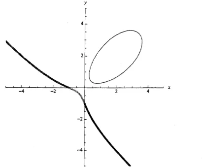
(see figure 1).

$y$

Figure 1: The real part ofthe Hesse cubic curve.

Each member of the pencil is denoted by $E_{t_{0},t_{1}}$ and the pencil itselfby $\{E_{t_{0},t_{1}}\}_{(t_{0},t_{1})\in \mathbb{P}^{1}(\mathbb{C})}$

.

The nine base points of the pencil aregiven as follows

$p_{0}=(0,1, -1)$ $p_{1}=(0,1, -\zeta_{3})$ $p_{2}=(0,1, -\zeta_{3}^{2})$

$p_{3}=(1,0, -1)$ $p_{4}=(1,0, -\zeta_{3}^{2})$ $p_{5}=(1,0, -\zeta_{3})$

$p_{6}=(1, -1,0)$ $p_{7}=(1, -\zeta_{3},0)$ $p_{8}=(1, -\zeta_{3}^{2},0)$,

where$\zeta_{3}$ denotes the primitive third root of1.

Any smooth curve in the pencil has the nine base points as its inflection points, and hence

they

are

intheHesseconfiguration [1, 8]. TheHesseconfiguration is anarrangement of 9 points

and 12lines in the projective plane $\mathbb{P}^{2}(\mathbb{C})$ which satisfies the following twoconditions;

.

eachline passes through three ofthe 9 points and

.

each point lies

on

four of the 12lines.

Once an elliptic

curve

is given then its 9 inflection points and 12 inflection

linesi

realize the

Hesse configuration. In particular, all non-singular members in the $Hess$ pencil have the 9

inflectionpoints$p_{0},p_{1},$ $\cdots,p_{8}$ andthe 12 inflection linesin common, henceeachofthem hasthe

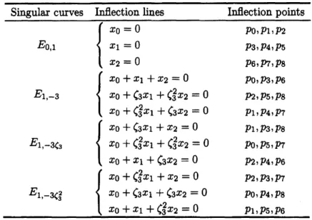
uniquerealizationof the Hesse configuration. Note that the 12 inflectionlinesaretheirreducible

components of the singular members$E_{0,1},$ $E_{1,-3},$ $E_{1,-3\zeta_{3}}$, and $E_{1,-\zeta_{3}^{2}}$ ofthe pencilgiven below

$\frac{(see(1-4))}{1A1inepasses}$

Table 1: Theinflection lines attd the inflection points in the

Hesse

configuration.

$\frac{Singu1arcurvesIfflectionlinesInflectionpoints}{E_{0,1}\{\begin{array}{l}x_{0}=0p_{0},p_{1},p_{2}x_{1}=0p_{3},p_{4},p_{5}x_{2}=0p_{6},p_{7},p_{8}\end{array}}$

$E_{1,-3}$ $\{\begin{array}{ll}x_{0}+x_{1}+x_{2}=0 p_{0},p_{3},p_{6}x_{0}+\zeta_{3}x_{1}+\zeta_{3}^{2}x_{2}=0 p_{2},p_{5},p_{8}\end{array}$

$E_{1,-3\zeta_{3}}$ $\{\begin{array}{ll}x_{0}+\zeta_{3}x_{1}+x_{2}=0 p_{1},p_{3},p_{8}x0+\zeta_{3}^{2}x_{1}+\zeta_{32}^{2_{X}}=0 p_{0},p_{5},p_{7}\end{array}$

$x_{0}+\zeta_{3}^{2}x_{1}+x_{2}=0$ $p_{2},p_{3},p_{7}$ $x_{0}+\zeta_{3}^{2}x_{1}+\zeta_{3}x_{2}=0$ $p_{1},p_{4},p_{7}$

$x0+x_{1}+\zeta_{3}x_{2}=0$ $p_{2},p_{4},p_{6}$

$E_{1,-3\zeta_{3}^{2}}$ $\{x_{0}+x_{1}+\zeta_{3}^{2}x_{2}=0$$x0+\zeta_{3}x_{1}+\zeta_{3}x_{2}=0$ $p0,p_{4},p_{8}$ $p_{1},p_{5},p_{6}$

The

WeierstraB

form of the Hesse cubic

curve

isgiven

as

foUows

$x_{1}^{!2}x_{2}’=x_{0}^{J3}+A(t_{0}, t_{1})x_{0}’x_{2}^{\prime 2}+B(t_{0}, t_{1})x_{2}^{l3}$,

where $(x_{0}’, x_{1}’, x_{2}’)\in \mathbb{P}^{2}(\mathbb{C})$ is the homogeneous coordinate of$\mathbb{P}^{2}(\mathbb{C}),$ _{$(t_{0}, t_{1})=(u_{0},6u_{1})$}, and

$A(t_{0}, t_{1})=12u_{1}(u_{0}^{3}-u_{1}^{3})$

$B(t_{0}, t_{1})=2(u_{0}^{6}-20u_{0}^{3}u_{1}^{3}-8u_{1}^{6})$

.

The transformation ${}^{t}(x_{0},$_{$x_{1},$}$x_{2})\mapsto{}^{t}(x_{0}’,$$x_{1}’,$$x_{2}’)$, form theHessefomto the WeierstraS3 form, is

givenby the linear map

$(-2\sqrt{6}it_{0}(27t_{0}^{3}9t_{0}t_{1}^{2}54t_{0}+t_{1}^{3})$ $2\sqrt{6}it_{0}(27t_{0}^{3}9t_{0}t_{1}^{2}54t_{0}+t_{1}^{3})$ $108t_{0}^{3}+t_{1}^{3}-18t_{1}0)$

.

The discriminant ofthe Weierstrai3cubic

curve

is

$\Delta=4A^{3}+27B^{2}=2^{2}3^{3}u_{0}^{3}(u_{0}^{3}+2^{3}u_{1}^{3})$

.

Thus we

see

that the singular memberof theHessepencil is describedby

$(t_{0}, t_{1})=(0,1),$ $(1, -3),$ $(1, -3\zeta_{3}),$ $(1, -3\zeta_{3}^{2})$,

or explicitly glven by the umions of threelines:

$E_{0,1}$ : $x_{0}x_{1}x_{2}=0$ (1)

$E_{1,-3}$ : $(x_{0}+x_{1}+x_{2})(x_{0}+\zeta_{3}x_{1}+\zeta i^{2_{X_{2}}})(+\alpha_{X)=0}$ (2)

$E_{1,-3\zeta_{3}}$ : $(x_{0}+\zeta_{3}x_{1}+x_{2})(x_{0}+\zeta_{3}^{2}x_{1}+\zeta_{3}^{2}x_{2})(x_{0}+x_{1}+\zeta_{3^{X}2})=0$ (3)

$E_{1,-3\zeta_{3}^{2}}$ : $(x_{0}+\zeta_{3}^{2}x_{1}+x_{2})(x_{0}+\zeta_{3}x_{1}+\zeta_{3}x_{2})(x_{0}+x_{1}+\zeta_{3}^{2}x_{2})=0$

.

(4)

Note that each singular member has multiplicity three. Table 1 shows the inflection lines and

2.2

Tropicalization

Let

us

consider tropicalization ofthe Hesse pencil, For the defining polynomial of the Hesse

cubic

curve

$f(x_{0}, x_{1}, x_{2};t_{0}, t_{1})$ $:=t_{0}(x_{0}^{3}+x_{1}^{3}+x_{2}^{3})+t_{1}x0x_{1}x_{2}$,

weapply the procedure of tropicalization. Atfirst, replacethe addition$+$and the multiplication

$\cross$ with the tropical addition $\oplus$ and the tropical multiplication $\otimes$ respectively; then we obtain

the tropical polynomial

$f(\overline{x}0,\tilde{x}_{1},\tilde{x}_{2};\tilde{t}_{0},\tilde{t}_{1})$ $:=\tilde{t}_{0}\otimes(\tilde{x}_{0}^{\otimes 3}\oplus\tilde{x}_{1}^{\otimes 3}\oplus\tilde{x}_{2}^{\otimes 3})\oplus\tilde{t}_{1}\otimes\tilde{x}_{0}\otimes\tilde{x}_{1}\otimes\tilde{x}_{2}$

.

In order to distinguish tropical variables form original ones, we ornament them with$\sim$

The

tropical operations $\oplus$and $\otimes$ aredefined as follows

$a \oplus b=\max(a, b)$ $a\otimes b=a+b$ for$a,$$b\in T:=$ RU$\{-\infty\}$,

where $T$is thetropical semi-field. Thus thetropical polynomial$f(\tilde{x}0,\tilde{X}_{1},\tilde{X}2;\tilde{t}_{0},\tilde{t}_{1})$ reduces to

$\tilde{f}(\tilde{x}0,\tilde{x}_{1},\tilde{x}_{2};\tilde{t}_{0},\tilde{t}_{1})=\max(\tilde{t}_{0}+3\tilde{x}0,\tilde{t}_{0}+3\tilde{x}_{1},\tilde{t}_{0}+3\tilde{x}_{2},\tilde{t}_{1}+\tilde{x}_{0}+\tilde{x}_{1}+\overline{x}_{2})$

.

Noting

$a\oplus(-\infty)=a$ $a\otimes 0=a$ $a\otimes(-a)=0$,

we

see

that-oo and$0$are theunitsofaddition and multiplicationin$T$respectively. Wefind the

element $-a$ as the inverse of$a$ with respect to the multiplication, however, there is no inverse

of$a$ with respect to the addition.

Definition 1 (See definition 1.1 in [5]) The tropical projective space $\mathbb{P}^{n,trop}$ consists of the

classes of $(n+1)$-tuples $(x_{0}, \cdots, x_{n})\in T^{n+1}$ such that not all ofthem

are

equal to $-$oo with

respect to the followingequivalencerelation $\sim$;

$(x_{0}, \cdots, x_{n})\sim(y_{0}, \cdots , y_{n})$ $\Leftrightarrow$ $x_{i}=y_{i}=\lambda$ for$i=0,$

$\ldots,$$n$and

$\lambda\in \mathbb{R}$,

wherewe assume $x_{0}\otimes\cdots\otimes x_{n}\neq-\infty$and $y_{0}\otimes\cdots\otimes y_{n}\neq-$oo.

Under the identification $(x_{1}, \ldots, x_{n})\in \mathbb{R}^{n}$ with $(0, x_{1}, \ldots, x_{n})\in \mathbb{P}^{n,trop}$ the real space $\mathbb{R}^{n}$ is

contained in $\mathbb{P}^{n,trop}$

.

Thus

we

have an embedding $\iota_{n}:\mathbb{R}^{n}\subset \mathbb{P}^{n,trop}$

.

Also we have $n+1$ affine

charts $T^{n}arrow \mathbb{P}^{n,trop}$, given by the (tropical) ratio with the j-th coordinate.

Let $(t_{0}, t_{1})$ be a point in $\mathbb{P}^{1,trop}$

.

Then $\tilde{f}$ can be regarded as a function $f:\mathbb{P}^{2,trop}arrow$ T.

The tropical Hesse

curve

is the set ofpoints such that the function $f$ is not differentiable. We

denote the tropical Hesse

curve

by $C_{\overline{t}_{0},\overline{t}_{1}}$

.

Upon introduction ofthe inhomogeneous coordinate

$(X :=\tilde{x}_{1}-\tilde{x}_{0}, Y:=\tilde{x}_{2}-\tilde{x}_{0})\in \mathbb{P}^{2,trop}$ and $K$ $:=\tilde{t}_{1}-\tilde{t}_{0}\in \mathbb{P}^{1,trop}$ the tropical Hesse curve is

denotedby $C_{K}$ and is given by thetropicalpolynomial

$F(X, Y;K)$ $:= \max(3X, 3Y, 0, K+X+Y)$

.

Figure2 shows the tropical Hesse curves. The one-dimensional linear system $\{C_{K}\}_{K\in P^{1,trop}}$

consistingofthetropicalHesse curvesis called the tropical Hesse pencil. The complement ofthe

tentacles,i.e., the finitepart,of$C_{K}$ isdenoted by$\overline{C}_{K}$. Wedenote the vertices whosecoordinates

are

$(K, K),$ $(-K, 0)$, and $(0, -K)$ by $V_{1},$ $V_{2}$, and $V_{3}$, respectively. Also denote theedges $\overline{V_{1}V_{2}}$, $\overline{V_{1}V_{2}}$, and$\overline{V_{1}V_{2}}$by_{$E_{1},$} $E_{2}$, and $E_{3}$, respectively.

$Y$

Figure2: Several members of the tropical Hesse pencil. The

ones

drawn withsolid lines

are

the

regular membersand theone with brokenline is the singular member for $K=0$

.

Each member $C_{K}$ of the tropical Hesse pencil for generic choice of $K\in \mathbb{P}^{1,trop}$ has genus

one, thereforeit

can

be regarded

as

a

tropicalellipticpencil. Singular

curves

appearonlyforthe

choice oftheparameter

as

$K=\infty$

or

$K\leq 0$

.

For$K=\infty$,

or

equivalentlyfor $(\tilde{t}_{0},\tilde{t}_{1})=(-$oo,$0)$,

the tropical polynomial $f(\overline{x}_{0},\tilde{x}_{1},\tilde{x}_{2};\tilde{t}_{0},\tilde{t}_{1})$ reduces to

$f(\tilde{x}_{0},\tilde{x}_{1},\tilde{x}_{2};-\infty, 0)=\tilde{x}_{0}\otimes\tilde{x}_{1}\otimes\tilde{x}_{2}=\tilde{x}_{0}+\tilde{x}_{1}+\tilde{x}_{2}$

.

(5)

This

can

not be

differentiated2

at theboundary of$\mathbb{P}^{2,tr\varphi}$, thereforethe

curve

$C_{K}$reducesto the

union of threetropical lines which compose the boundary of$\mathbb{P}^{2,trop}$:

$C_{\infty}$ : $\{\tilde{x}_{0}=-\infty\}\cup\{\tilde{x}_{1}=-oo\}\cup\{\tilde{x}_{2}=-oo\}$

.

(6)

Sincethe defining polynomial of the singular

curve

$E_{0,1}$ is

$f(x_{0}, x_{1}, x_{2};0,1)=x_{0}x_{1}x_{2)}$ (7)

the tropical polynomial (5)

can

be regarded

as

thetropicalizationof(7). Therefore, thesingular

curve

$C_{\infty}$ is the tropical counterpart of$E_{0,1}$

.

Ontheother hand, for$K\leq 0$, orequivalently for$\tilde{t}_{0}\geq\tilde{t}_{1},$ $F(X, Y;K)$ reduces to

$F(X, Y;K)=3\max(X, Y, 0)$, (8)

orequivalently $f(\tilde{x}_{0},\tilde{x}_{1},\tilde{x}_{2};\tilde{t}_{0},\tilde{t}_{1})$ to

$\tilde{f}(\tilde{X}_{0},\tilde{X}_{1},\tilde{X}2;\tilde{t}_{0},\tilde{t}_{1})=(\tilde{x}_{0}\oplus\overline{x}_{1}\oplus\tilde{x}_{2})^{\otimes 3}=3\max(\tilde{x}_{0},\tilde{x}_{1},\tilde{x}_{2})$

.

(9)

2Forexample,for fixed$\tilde{x}_{1},\tilde{x}_{2}\in T$and$h>0$,thedifference

$\{\overline{f}(-\infty+h,\tilde{x}_{1},\overline{x}_{2};-\infty, 0)-\tilde{f}(-oo, \tilde{x}_{1},\tilde{x}_{2};-oo, 0)\}/h$

The tropical

curve

given by (8) is clearly independentof$K$

.

Hence we take $C_{0}$ as the

represen-tative of the singular

curves

$C_{K}$ for$K\leq 0$

.

The

curve

$C_{0}$ is

a

triple tropical line whose only

vertex is

on

the origin (seefigure2). The tropical polynomial (9)

can

be regardedas the

tropi-calization ofthepolynomials in (2), (3), and (4), whichgive the singular

curves

$E_{1,-3},$ $E_{1,-3\zeta_{3}}$,

and $E_{1,-3\zeta_{3}^{2}}$, respectively. Thus the curve $C_{0}$ is regarded

as

the tropical counterpart of_{$E_{1,-3}$}, $E_{1,-3\zeta_{3}}$, and $E_{1,-3\zeta_{3}^{2}}$

.

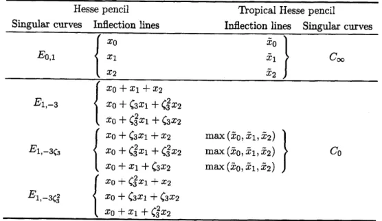
Table2 showsthe correspondence betweenthe definingpolynomialsofthe

singularmembers of the Hessepencil and their tropical counterparts.

Table 2: The correspondence _{between the defining polynomials of the singular members of the}

Hessepencil _{and their tropical counterparts.}

Hesse pencil TkopicalHessepencil

Singular

curves

Inflectionlines Inflection lines Singular

curves

$E_{0,1}$ $\{\begin{array}{ll}x_{0} \tilde{x}_{0}x_{1} \overline{x}_{1}x_{2} \tilde{x}_{2}\end{array}\}$ $C_{\infty}$

$\overline{E_{1,-3}\{\begin{array}{l}x_{0}+x_{1}+x_{2}xo+\zeta_{3}x_{1}+\zeta_{3}^{2}x_{2}x_{0}+\zeta_{3}^{2}x_{1}+\zeta_{3}x_{2}\end{array}}$

$E_{1,-3\zeta_{3}}$ $\{\begin{array}{ll}xo+\zeta_{3}x_{1}+x_{2} \max(\tilde{x}_{0},\tilde{x}_{1},\tilde{x}_{2})x_{0}+\zeta_{3}^{2}x_{1}+\zeta_{3}^{2}x_{2} \max(\tilde{x}_{0},\overline{x}_{1,2}\tilde{x})x_{0}+x_{1}+\zeta_{3}x_{2} \max(\tilde{x}_{0},\tilde{x}_{1},\tilde{x}_{2})\end{array}\}$ $C_{0}$

$x0+\zeta_{3}x_{1}+\zeta_{3}x_{2}$

$\underline{E_{1,-3\zeta_{3}^{2}}\{\begin{array}{l}x_{0}+\zeta_{3}^{2}x_{1}+x_{2}x_{0}+x_{1}+\zeta_{3}^{2}x_{2}\end{array}}$

Vigeland showed that atropical elliptic

curve

has an additivegroup structurein analogy to

an elliptic

curve

[9]. The group structureis induced from that ofthe Jacobian ofthe tropical

elliptic curve, which is isomorphic to $S^{1}$, to its complement ofthe tentaclesvia the

Abel-Jacobi

map. Therefore wehave the group isomorphism

$\overline{C}_{K}\simeq C_{K}/\simarrow J(C_{K})\simeq S^{1}$,

where $\sim$ is

an

equivalence relation called the linear

equivalence [9]. In thefollowing, we givean

explicit_{formula for the additionof pointsonthetropicalHesse curveviathe ultradiscretization}

ofthose for thelevel-three theta functions.

3

_{Level-three theta}

_functions

3.1

Definition

The level-three theta functions $\theta_{0}(z, \tau),$ $\theta_{1}(z, \tau)$, and $\theta_{2}(z, \tau)$

are

defined by using the theta

function$\theta_{(a,b)}(z, \tau)$ with characteristics:

where $z\in \mathbb{C}$and$\tau\in \mathbb{H}$ $:=\{\tau\in \mathbb{C}|{\rm Im}\tau>0\}$

.

Fix $\tau\in$IHI. For simplicity,

we

abbreviate $\theta_{k}(z,\tau)$ and $\theta_{k}(0, \tau)$

as

$\theta_{k}(z)$ and $\theta_{k}$ for $k=0,1,2$,

respectively. The level-three thetafunctions havethequasiperiodicity [3]

$\theta_{k}(z+1)=-\theta_{k}(z)$ (10)

$\theta_{k}(z+\tau)=-e^{3\pi i\tau}e^{-6\pi iz}\theta_{k}(z)$ (11)

for $k=0,1,2$

.

Let $L_{\tau}$ $:=(-\tau)Z+(3\tau+1)Z$be

a

lattice in

C.

Noting

$(\begin{array}{ll}-l 30 l\end{array})=(\begin{array}{ll}-l 30 l\end{array})$

wehave

an

isomorphism$L_{\tau}\simeq \mathbb{C}/Z+\tau Z$

.

Let

us

denote the

axes

in the$directions-\tau$ and$3\tau+1$

$’$ ’ $’\backslash$’ $\backslash s$ $’$ ’ $\backslash$ $\nu’$ $O$

Figure 3: The

zeros

of$\theta_{k}(z, \tau)$ for $k=0,1,2$ in the fundamental domain.

by$a$ and $b$respectively (see figure 3).

3.2

Addition formulae

Theorem 1 For

a

fixed $\tau\in$ IE, the level-three theta functions $\theta_{0}(z, \tau),$ $\theta_{1}(z, \tau)$, and $\theta_{2}(z, \tau)$

satisfy thefollowing 9 functional relations calledthe additionformulae [3]

$\theta_{0}^{2}\theta_{0}(z+w)\theta_{0}(z-w)=\theta_{1}(z)\theta_{2}(z)\theta_{2}(w)^{2}-\theta_{0}(z)^{2}\theta_{0}(w)\theta_{1}(w)$ (12a) $\theta_{0}^{2}\theta_{1}(z+w)\theta_{0}(z-w)=\theta_{0}(z)\theta_{1}(z)\theta_{1}(w)^{2}-\theta_{2}(z)^{2}\theta_{0}(w)\theta_{2}(w)$ (12b) $\theta_{0}^{2}\theta_{2}(z+w)\theta_{0}(z-w)=\theta_{0}(z)\theta_{2}(z)\theta_{0}(w)^{2}-\theta_{1}(z)^{2}\theta_{1}(w)\theta_{2}(w)$ (12c) $\theta_{0}^{2}\theta_{0}(z+w)\theta_{1}(z-w)=\theta_{0}(z)\theta_{1}(z)\theta_{0}(w)^{2}-\theta_{2}(z)^{2}\theta_{1}(w)\theta_{2}(w)$ (13a) $\theta_{0}^{2}\theta_{1}(z+w)\theta_{1}(z-w)=\theta_{0}(z)\theta_{2}(z)\theta_{2}(w)^{2}-\theta_{1}(z)^{2}\theta_{0}(w)\theta_{1}(w)$ (13b) $\theta_{0}^{2}\theta_{2}(z+w)\theta_{1}(z-w)=\theta_{1}(z)\theta_{2}(z)\theta_{1}(w)^{2}-\theta_{0}(z)^{2}\theta_{0}(w)\theta_{2}(w)$ (13c) $\theta_{0}^{2}\theta_{0}(z+w)\theta_{2}(z-w)=\theta_{0}(z)\theta_{2}(z)\theta_{1}(w)^{2}-\theta_{1}(z)^{2}\theta_{0}(w)\theta_{2}(w)$ (14a) $\theta_{0}^{2}\theta_{1}(z+w)\theta_{2}(z-w)=\theta_{1}(z)\theta_{2}(z)\theta_{0}(w)^{2}-\theta_{0}(z)^{2}\theta_{1}(w)\theta_{2}(w)$ (14b) $\theta_{0}^{2}\theta_{2}(z+w)\theta_{2}(z-w)=\theta_{0}(z)\theta_{1}(z)\theta_{2}(w)^{2}-\theta_{2}(z)^{2}\theta_{0}(w)\theta_{1}(w)$ , (14c) where$z,$$w\in$C.

It follows from theorem 1 that

we

have [3]

$\theta_{2}’(\theta_{0}(z)^{3}+\theta_{1}(z)^{3}+\theta_{2}(z)^{3})+6\theta_{0}’\theta_{0}(z)\theta_{1}(z)\theta_{2}(z)=0$

.

(15)

Consider amap $\varphi$ : $\mathbb{C}arrow \mathbb{P}^{2}(\mathbb{C})$,

$\varphi:z\mapsto(\theta_{2}(z), \theta_{0}(z), \theta_{1}(z))$

.

This induces amap $hom$ _{the complex torus}$\mathbb{C}/L_{\tau}$ totheHesse cubic

curve

$E_{\theta_{2}’,6\theta_{0}’}$ due to (10),

(11), and (15). This mapisknowntogive

an

isomorphism$\mathbb{C}/L_{\tau}\simeq E_{\theta_{2}’,6\theta_{0}’}$

.

Thus the level-three

thetafunctions parametrize the Hesse cubic curve.

Considering $(12a-12c)$, the point $(\theta_{2}(z+w), \theta_{0}(z+w), \theta_{1}(z+w))$ is computed

as

follows

$(\theta_{2}(z+w), \theta_{0}(z+w), \theta_{1}(z+w))=(\theta_{0}(z)\theta_{2}(z)\theta_{0}(w)^{2}-\theta_{1}(z)^{2}\theta_{1}(w)\theta_{2}(w)$, $\theta_{1}(z)\theta_{2}(z)\theta_{2}(w)^{2}-\theta_{0}(z)^{2}\theta_{0}(w)\theta_{1}(w)$ ,

$\theta_{0}(z)\theta_{1}(z)\theta_{1}(w)^{2}-\theta_{2}(z)^{2}\theta_{0}(w)\theta_{2}(w))$ (16)

except for $z,$$w\in \mathbb{C}/L_{\tau}$ satisfying _{$\theta_{0}(z-w)=0$}

.

Similarly, considering $(13a-13c)$ and $(14a-$

$14c)$,

we

obtain the following

$(\theta_{2}(z+w), \theta_{0}(z+w), \theta_{1}(z+w))=(\theta_{1}(z)\theta_{2}(z)\theta_{1}(w)^{2}-\theta_{0}(z)^{2}\theta_{0}(w)\theta_{2}(w)$ , $\theta_{0}(z)\theta_{1}(z)\theta_{0}(w)^{2}-\theta_{2}(z)^{2}\theta_{1}(w)\theta_{2}(w)$,

$\theta_{0}(z)\theta_{2}(z)\theta_{2}(w)^{2}-\theta_{1}(z)^{2}\theta_{0}(w)\theta_{1}(w))$ (17) $(\theta_{2}(z+w), \theta_{0}(z+w), \theta_{1}(z+w))=(\theta_{0}(z)\theta_{1}(z)\theta_{2}(w)^{2}-\theta_{2}(z)^{2}\theta_{0}(w)\theta_{1}(w)$ ,

$\theta_{0}(z)\theta_{2}(z)\theta_{1}(w)^{2}-\theta_{1}(z)^{2}\theta_{0}(w)\theta_{2}(w)$,

$\theta_{1}(z)\theta_{2}(z)\theta_{0}(w)^{2}-\theta_{0}(z)^{2}\theta_{1}(w)\theta_{2}(w))$ (18)

exceptfor $z,$$w\in \mathbb{C}/L_{\tau}$ satisfying $\theta_{1}(z-w)=0$ and$\theta_{2}(z-w)=0$, respectively. Sincethe

zeros

of$\theta_{0}(z),$ $\theta_{1}(z)$, and $\theta_{2}(z)$

never

coincide with eachother, at least two of the additionformulae

(16–18)canbe definedforany$z,$$w\in \mathbb{C}/L_{\tau}$

.

Moreover, by using the relation (15),

we

canprove

that thethree formulae(16-18)

are

essentially the

same

where theyaredefined simultaneously.

Thus theaddition formulaforthe Hesse cubic

curve

is uniquely defined

on

$\mathbb{C}/L_{\tau}$

.

The isomorphism $\varphi$ : $\mathbb{C}/L_{\tau}arrow E_{\theta_{2}’,6\theta_{0}^{l}}$ induces the additive group structure on $E_{\theta_{2}’,6\theta_{0}’}$ from

$\mathbb{C}/L_{\tau}$ throughthe addition formulae for the level-three theta functions. The relation (19) (see

below) implies

$\varphi:0\mapsto(\theta_{2}, \theta_{0}, \theta_{1})=(0,1, -1)=p_{0}$

.

Thus

we

obtain the addition formulae for the Hesse cubic

curve

$(E_{\theta_{2}’,6\theta_{\acute{0}}},p_{0})$ equipped with the

unit ofaddition$p_{0}$

.

Theorem 2 Let the unit of addition

on

the Hesse cubic

curve

$E_{\theta_{2}’,6\theta_{0}’}$ be$p0=(0,1, -1)$

.

Let $(x_{0}, x_{1}, x_{2})$ and $(x_{0}’, x_{1}’, x_{2}’)$ be points on$E_{\theta_{2}’,6\theta_{0}’}$

.

Then the addition $(x_{0}, x_{1}, x_{2})+(x_{0}’, x_{1}’, x_{2}’)$ of

thepoints aregiven

as

follows

$(x_{0}, x_{1}, x_{2})+(x_{0}’, x_{1}’, x_{2}’)=(x_{1}x_{2}x_{2}^{;2}-x_{0}^{2}x_{0}’x_{1}’, x_{0}x_{1}x_{1^{2}}’-x_{2}^{2}x_{0}’x_{2}’, x_{0}x_{2}x_{0^{2}}’-x_{1}^{2}x_{1}’x_{2}’)$ $=(x_{0}x_{1}x_{0^{2}}’-x_{2}^{2}x_{1}^{l}x_{2}’, x_{0}x_{2}x_{2}^{\prime 2}-x_{1}^{2}x_{0}’x_{1}’, x_{1}x_{2}x_{1^{2}}’-x_{0}^{2}x_{0}’x_{2}’)$

We

can

easily

see

that the following property holds

$\theta_{0}=-\theta_{1}$ $\theta_{2}=0$ (19)

$\theta_{k}(Z+\frac{\tau}{3})5^{\pi i\tau}$ (20)

$\theta_{k}(Z+\frac{1}{3})=e^{2\pi i(_{F^{-}\delta}^{k1})_{\theta_{k}(z)}}$

.

(21)

The relations (19–21) imply that

we can

take the following representatives $z_{0k,k1k2}z,$$z$ of the

zeros

of$\theta_{k}(z)$ in $\mathbb{C}/L_{\tau}$ for $k=0,1,2$ (seefigure3)

$(\begin{array}{lll}z_{20} z_{21} z22z_{00} z_{01} zo2z_{10} z_{11} z_{12}\end{array})=(\begin{array}{lll}0 \tau+51 2\tau+\frac{2}{3}-5\tau \frac{2\tau}{3}+51 \frac{5\tau}{3}+\frac{2}{3}-T F^{+}5\tau 1 T+F4\tau 2\end{array})$

.

These nine

zeros

are

mappedinto the nine inflection points on$E_{\theta_{2}’,6\theta_{\acute{0}}}$ by$\varphi$, respectively:

$z_{20}$ $z_{21}$ $z_{22}$ $p0$ $p_{1}$ $p_{2}$

$\varphi$ :

$z_{10}z_{00}$ $z_{11}z_{01}$ $z_{12}z_{02}$ $p_{6}p_{3}$ $p_{7}p_{4}$ $p_{8}p_{5}$

.

(22)

4

Addition formula for

the tropical

Hesse

pencil

4.1

Parametrization

of the complex

torus

In [3], weapplytheprocedureofultradiscretization to the level-threetheta functions, and obtain

piecewise linear functions which parametrize the complement of the tentacles of the tropical

Hesse

curve.

We recall the result here.

Let $K$ and$\epsilon$ be positivenumbers. Let

us

fix$\tau$

as

follows

$\tau=-\frac{3K}{9K+2\pi i\epsilon}$

.

(23)

For thischoice of$\tau$, a point $z\in \mathbb{C}/L_{\tau}$ iswritten

as

follows

$z=(-\tau)a+(3\tau+1)b$

$= \frac{3Ka}{9K+2\pi i\epsilon}+\frac{2\pi i\epsilon b}{9K+2\pi i\epsilon}$, (24)

where$0\leq a,$$b<1$

.

Introducingsuch a new variable$u\in \mathbb{R}$that

$a= \frac{u}{3K}(1+\xi_{\epsilon}^{2})$ ,

where$\xi_{\epsilon}=2\pi\epsilon/9K,$ (24) reduces to

$z= \frac{(1-i\xi_{\epsilon})u}{9K}+\frac{i\xi_{\epsilon}b}{1+i\xi_{\epsilon}}$

.

(25)

Since $0\leq a<1$, wehave

Ifwe take the limit $\epsilonarrow 0$ then

we

have

$\tauarrow-\frac{1}{3}$, $\xi_{\epsilon}arrow 0$, and $z arrow\frac{u}{9K}$

.

Hence weobtain

$z_{20}$ $z_{21}$ $z_{22}$ $0$ $0$ $0$

$z_{10}z_{00}$ $z_{11}z_{01}$ $z_{12}z_{02}$ $arrow$

$\frac{\frac{1}{29}}{9}$ $\frac{\frac{1}{29}}{9}$ $\frac{1}{\frac 29,9}$

$(\epsilonarrow 0)$

.

In termsof the variable $u$,

we

put the limit of

zeros

$z_{kj}(k,j=0,1,2)$

as

follows

$u_{2}$ _{$:= \lim_{\epsilonarrow 0}9Kz_{20}=\lim_{\epsilonarrow 0}9Kz_{21}=\lim_{earrow 0}9Kz_{22}=0$} (27)

$u_{0}:= \lim_{\epsilonarrow 0}9Kz_{00}=\lim_{\epsilonarrow 0}9Kz_{01}=\lim_{\epsilonarrow 0}9Kz_{02}=K$ (28)

$u_{1}$ _{$:=!_{arrow 0}^{im9Kz_{10}}= \lim_{\epsilonarrow 0}9Kz_{11}=\lim_{\epsilonarrow 0}9Kz_{12}=2K$}

.

(29)

Let usconsider aline $l_{\epsilon}$ in $\mathbb{C}$ along with the a-axis

$l_{\epsilon}= \{\frac{(1-i\xi_{\epsilon})u}{9K}|u\in \mathbb{R}\}$

.

Then the circle $l_{\epsilon}/\tau Z$is contained in the complex torus $\mathbb{C}/L_{\tau}$

.

We define thetropicalJacobian

$J(C_{K})$ of thetropical Hesse

curve

$C_{K}$

as

follows

$\lim_{\epsilonarrow 0}l_{\epsilon}/\tau Z\simeq \mathbb{R}/3KZ=\{u\in \mathbb{R}|0\leq u<3K\}=:J(C_{K})$

.

Proposition 1 Let $\tau$ be

as

in (23). Then thecomplextorus $\mathbb{C}/L_{\tau}$convergesinto $J(C_{K})$ inthe

limit $\epsilonarrow 0$ with respectto theHausdorffmetric.

(Proof) Let the point $z\in \mathbb{C}/L_{\tau}$be

as

in (25). Then

$\inf_{v\in J(C_{K})}d(9Kz, J(C_{K}))\leq d(9Kz, u)$

$=|-iu+ \frac{9Kib}{1+i\xi_{\epsilon}}|\xi_{\epsilon}$

$<M\epsilon$

forsome $M>0$_{. Similarly, for sufficiently small} $\epsilon>0$, it follows form (26) that wehave

$v< \frac{3K}{1+\xi_{\epsilon}}$

for any$v\in J(C_{K})$, and hence

we can

take such $z$ that

$z= \frac{(1-i\xi_{\epsilon})v}{9K}+\frac{i\xi_{\epsilon}b}{1+i\xi_{\epsilon}}$

.

Thus we have

$\inf_{z\in \mathbb{C}/L_{\tau}}d(\mathbb{C}/L_{\tau}, v)\leq d((1-i\xi_{\epsilon})v+\frac{9Ki\xi_{\epsilon}b}{1+i\xi_{\epsilon}},$$v)$

$=|-iv+ \frac{9Kib}{1+i\xi_{\epsilon}}|\xi_{\epsilon}$

$<M’\epsilon$

.

4.2

Ultradiscretization

Now we show that the points on the a-axis in the complex torus $\mathbb{C}/L_{\tau}$ correspond to that

on

the real part oftheHesse cubic

curve.

Proposition 2 Let $\tau$be

as

in (23). Then $\varphi$ mapsthe points on the circle $l_{\epsilon}/\tau Z$into $E_{\theta_{2}’,6\theta_{0}’}\cap$

$\mathbb{P}^{2}(\mathbb{R})$, the real part ofthe Hesse cubic

curve.

(Proof) By using the formula concerning the modular transformation of the level-three

theta functions (see proposition 4.3 in [3]),we have

$\theta_{k}(z, \tau)=e^{\frac{-9\pi 1z^{2}}{3\tau+1}}(3\tau+1)^{-}\tau_{e}\tau^{\underline{j}}\theta_{(_{3^{-}8’ l}^{k73})}1\pi(\frac{3z}{3\tau+1’}\frac{3\tau}{3\tau+1})\cdot$

Since $z$ isassumed to be on $l_{\epsilon}/\tau Z$, we

can

put $z$ be

as

in (25) with $b=0$

.

Then weobtain

$\theta_{(\frac{k}{3}-\epsilon,z)}73(\frac{3z}{3\tau+1},$$\frac{3\tau}{3\tau+1})=(-1)^{k}i^{u^{2}}eR$

$\cross\sum_{n\in Z}\exp[(n+\frac{k}{3}-\frac{7}{6})\frac{3\xi_{e}^{2}}{\epsilon}u-\frac{9K}{2\epsilon}(\frac{u-(k+1)K}{3K}-n+\frac{3}{2})^{2}](-1)^{n}$

.

(30)

The imaginarypart ofthe functions $\theta_{0}(z,\tau),$ $\theta_{1}(z, \tau)$, and $\theta_{2}(z, \tau)$ appear only in the following

common factor

$e \frac{-9\pi z^{2}}{3\tau+1}(3\tau+1)^{-}ze^{\frac{\pi t}{4}}i1$

.

Therefore,

we

have $\varphi(z)\in E_{\theta_{2}’,6\theta_{0}’}\cap \mathbb{P}^{2}(\mathbb{R})$

.

$\blacksquare$

There exist three

zeros

$z_{20},$ $z_{00}$, and$z_{10}$of the level-three theta functions

on

$l_{\epsilon}/\tau Z$(seefigure

3$)$

.

These

zeros

divide$l_{\epsilon}/\tau Z$ into three open intervalsdenoted by$d_{1},$ $d_{2}$, and $d_{3}$:

$d_{j}:= \{-\tau a\in \mathbb{C}/L_{\tau}|\frac{j-1}{3}<a<\frac{j}{3}\}$

$= \{\frac{(1-i\xi_{\epsilon})}{9K}u\in \mathbb{C}/L_{\tau}|\frac{(j-1)K}{1+\xi_{\text{\’{e}}}^{2}}<u<\frac{jK}{1+\xi_{\epsilon}^{2}}\}$ $(j=1,2,3)$

.

Noticing (22), wehave

$\varphi(z_{20})=p_{0}=(\infty, \infty)$, $\varphi(z_{00})=p_{3}=(0, -1)$, $\varphi(z_{10})=p_{6}=(-1,0)$

in the inhomogeneous coordinate $(x :=x_{1}/x_{0}, y :=x_{2}/x_{0})$ of$\mathbb{P}^{2}(\mathbb{C})$, and hence

we

obtain the

following (seefigure 1)

$\varphi(d_{1})=\{(x, y)\in E_{\theta_{2}’,w_{0}}\cap \mathbb{P}^{2}(\mathbb{R})|x>0,$ $y<0\}$ (31) $\varphi(d_{2})=\{(x, y)\in E_{\theta_{2}’,6\theta_{\acute{0}}}\cap \mathbb{P}^{2}(\mathbb{R})|x<0,$ $y<0\}$ (32) $\varphi(d_{3})=\{(x, y)\in E_{\theta_{2}’,6\theta_{0}’}\cap \mathbb{P}^{2}(\mathbb{R})|x<0,$ $y>0\}$

.

(33)

We define the open subsets$D_{1},$ $D_{2}$, and$D_{3}$ of $J(C_{K})$

as

follows

$D_{j}$ _{$:= \lim_{\epsilonarrow 0}d_{j}=\{u\in J(C_{K})|(j-1)K<u<jK\}$} $(j=1,2,3)$

.

Then wehave$J(C_{K})= \bigcup_{j=0}^{2}(D_{j+1}\cup u_{j})$, where$uk\equiv(k+1)K(mod 3)$ is the limiting pointof

Next weconsider the amoeba of the real part of$E_{\theta_{2}’,6\theta_{0}’}$ which is defined

as

the set ofpoints $(\epsilon\log|x|, \epsilon\log|y|)$ satisfying$(x, y)\in E_{\theta_{2}’,6\theta_{\acute{0}}}\cap \mathbb{P}^{2}(\mathbb{R})$. Let $z$ beapoint

on

theopenset $d_{1}\cup d_{2}\cup d_{3}$

.

Then wehave $\theta_{k}(z)\neq 0$for$k=0,1,2$

.

Since $(x, y)=\varphi(z)=(\theta_{0}(z)/\theta_{2}(z), \theta_{1}(z)/\theta_{2}(z))$, wehave

(see (30))

$\epsilon\log|x|=\epsilon\log|\frac{\theta_{0}(z)}{\theta_{2}(z)}|$

$= \epsilon\log|\frac{\sum_{n\in Z}\exp[(n-\frac{7}{6})\frac{3\xi_{\epsilon}^{2}}{\epsilon}u-\frac{9K}{2\epsilon}(\frac{u-K}{3K}-n+\frac{3}{2})^{2}](-1)^{n}}{\sum_{n\in Z}\exp[(n-\frac{1}{2})\frac{3\xi_{\epsilon}^{2}}{\epsilon}u-\frac{9K}{2\epsilon}(\frac{u-3K}{3K}-n+\frac{3}{2})^{2}](-1)^{n}}|$

and

$\epsilon\log|y|=\epsilon\log|\frac{\theta_{1}(z)}{\theta_{2}(z)}|$

$= \epsilon\log|\frac{\sum_{n\in Z}\exp[(n-\frac{5}{6})\frac{3\xi_{\epsilon}^{2}}{\epsilon}u-\frac{9K}{2\epsilon}(\frac{u-2K}{3K}-n+\frac{3}{2})^{2}](-1)^{n}}{\sum_{n\in Z}\exp[(n-\frac{1}{2})\frac{3\xi_{\epsilon}^{2}}{\epsilon}u-\frac{9K}{2\epsilon}(\frac{u-3K}{3K}-n+\frac{3}{2})^{2}](-1)^{n}}|$

.

Define thepiecewise linearfunctions

$\tilde{c}(u):=-\frac{9K}{2}\{((\frac{u-K}{3K}-\frac{1}{2}))\}^{2}+\frac{9K}{2}\{$ $(( \frac{u-3K}{3K}-\frac{1}{2}))\}^{2}$

$\tilde{s}(u):=-\frac{9K}{2}\{((\frac{u-2K}{3K}-\frac{1}{2}))\}^{2}+\frac{9K}{2}\{$$(( \frac{u-3K}{3K}-\frac{1}{2}))\}^{2}$

where thefunction $($( )$)$ :$\mathbb{R}arrow[0,1)$ is defined as follows

$((u))=u-$Floor$(u)$.

Also definethe subset $R\subset \mathbb{R}$

$R:= \bigcup_{j=1}^{3}\{a\in \mathbb{R}|\frac{j-1}{3}<a<\frac{j}{3}\}$

.

Then weobtain thefollowing proposition.

Proposition 3 Let $\tau$be as in (23). Assume $a\in R$

.

Then thefunctions

$\epsilon\log|\frac{\theta_{0}(-a\tau)}{\theta_{2}(-a\tau)}|$ and $\epsilon\log|\frac{\theta_{1}(-a\tau)}{\theta_{2}(-a\tau)}|$ (34)

uniformly converge into

$\tilde{c}(3Ka)$ and $\tilde{s}(3Ka)$ (35)

(Proof) By proposition 2, $\varphi(z)$ is

a

point

on

the real part of $E_{\theta_{2}’,6\theta_{0}’}$ for $z\in\{-a\tau|0\leq$

$a<1\}$

.

Let $\delta$ be

an

arbitrary positive number less than 1/6. Then

we

can

take $a$ $SatIS\mathfrak{h}ring$ $j/3+\delta\leq a\leq(j+1)/3-\delta$ for any $j\in\{0,1,2\}$

.

For this choice of $a$,

we

have $-a\tau\in d_{j}$,

and hence $\theta_{k}(-a\tau)(k=0,1,2)$ does not vanish. Thus

we

can

define the functions (34)

on

the

compact set

$R_{\delta}:= \bigcup_{j=1}^{3}\{a\in \mathbb{R}|\frac{j-1}{3}+\delta\leq a\leq\frac{j}{3}-\delta\}$

.

Ifwe take $a$

as

above, then

we

have$jK+3K\delta\leq 3Ka\leq(j+1)K-3K\delta$, and hence $3Ka$ is

contained in $D_{j}$ becauseof the assumption $0<\delta<1/6$

.

Thus the functions (35)

can

also be

defined

on

$R_{\delta}$

.

We canestimate $\theta_{0}(-a\tau)$

as

follows. Put

$m=n-n_{0}(u)$, $n_{0}(u)=$ Floor $( \frac{u-K}{3K})+2$

.

Then we have $\sum_{n\in Z}\exp[(n-\frac{7}{6})\frac{3\xi_{\epsilon}^{2}}{\epsilon}u]\exp[-\frac{9K}{2\epsilon}(\frac{u-K}{3K}-n+\frac{3}{2})^{2}](-1)^{n}$ $= \sum_{m\in Z}\exp[(m+n_{0}(u)-\frac{7}{6})\frac{3\xi_{\epsilon}^{2}}{\epsilon}u]\exp[-\frac{9K}{2\epsilon}\{((\frac{u-K}{3K}))-m-\frac{1}{2}\}^{2}](-1)^{m+no(u)}$ $= \exp[-\frac{9K}{2\epsilon}\{((\frac{u-K}{3K}))-\frac{1}{2}\}^{2}+(n_{0}(u)-\frac{7}{6})\frac{3\xi_{\epsilon}^{2}}{\epsilon}u](-1)^{no(u)}$ $\cross\sum_{m\in Z}\exp[-\frac{9K}{2\epsilon}\{m+1-2((\frac{u-K}{3K}))-\frac{2\xi_{\epsilon}^{2}}{3K}u\}m](-1)^{m}$

.

for $m>>0$

Noting$u\in D_{1}\cup D_{2}\cup D_{3}$, for sufficientlysmall $\epsilon$, we have

$- \frac{9K}{2\epsilon}\{m+1-2((\frac{u-K}{3K}))-\frac{2\xi_{\epsilon}^{2}}{3K}u\}<0$

for $m<<0$

.

$- \frac{9K}{2\epsilon}\{m+1-2((\frac{u-K}{3K}))-\frac{2\xi_{\epsilon}^{2}}{3K}u\}>0$

exceptfor finite $m\in$ Z.

Hence, for any$u\in D_{1}\cup D_{2}\cup D_{3}$, there exists such$0<r<1$ that $\exp[-\frac{9K}{2\epsilon}\{m+1-2((\frac{u-K}{3K}))-\frac{2\xi_{\epsilon}^{2}}{3K}u\}m]<r^{|m|}$

Therefore, wehave

$\epsilon\log|\theta_{0}(-a\tau)|=-\frac{9K}{2}\{((\frac{u-K}{3K}))-\frac{1}{2}\}^{2}+o(1)$

.

Similarly, for$\theta_{2}(-a\tau)$, we have

$\epsilon\log|\theta_{2}(-a\tau)|=-\frac{9K}{2}\{((\frac{u-3K}{3K}))-\frac{1}{2}\}^{2}+o(1)$

.

Thus the function$\epsilon\log|\theta_{0}(-a\tau)/\theta_{2}(-a\tau)|$ uniformly converges into $\tilde{c}(3Ka)$ in the limit $\epsilonarrow 0$

The piecewise linearfunctions $\tilde{c}$ and $\tilde{s}$

are

defined

on

$\bigcup_{j=1}^{3}D_{j}=J(C_{K})\backslash \{u_{0}, u_{1}, u_{2}\}$

.

Ifwe

extend them to be continuous functions

on

$J(C_{K})$ then their values

on

the points _{$u_{2},$ $u_{0},$}$u_{1}$

are

uniquely determinedas follows

$\tilde{c}(u_{2})=K$ $\tilde{c}(u_{0})=-K$ $\tilde{c}(u_{1})=0$

$\tilde{s}(u_{2})=K$ $\tilde{s}(u_{0})=0$ $\tilde{s}(u_{1})=-K.$ (36)

The extended continuouspiecewise linear functions

are

also denoted by$\tilde{c}$and $\tilde{s}$ (seefiguues4(a) and $4(b))$

.

Note that the_points $u_{2},$ $u_{0},$$u_{1}$

are

mapped into the vertices of$\overline{C}_{K}$:

$(\tilde{c}(u_{2}),\tilde{s}(u_{2}))=V_{1}$, $(\tilde{c}(u_{0}),\tilde{s}(u_{0}))=V_{2}$, $(\tilde{c}(u_{1}),\tilde{s}(u_{1}))=V_{3}$

.

$\overline{c}(u)$ $u$ $0$ $K$ $2K$ $3K$ (a) $\tilde{s}(u)$ $u$ $0$ $K$ $2K$ $3K$ (b)

Figure4: (a) $\tilde{c}:J(C_{K})arrow \mathbb{R}$

.

(b) $\tilde{s}:J(C_{K})arrow \mathbb{R}$

.

Let us introduce a map$\tilde{\varphi}$ : $J(C_{K})arrow \mathbb{R}^{2}\subset \mathbb{P}^{2,trop}$,

$\tilde{\varphi}$ : $u(\tilde{c}(u),\tilde{s}(u))$

.

(37) This map induces

an

isomorphism $J(C_{K})\simeq\overline{C}_{K}$

.

Therefore, we have

$\{(\tilde{c}(u),\tilde{s}(u))\in \mathbb{R}^{2}|u\in J(C_{K})\}=\overline{C}_{K}$

.

Thusweobtain thepiecewiselinear functions$\tilde{c}(u)$ and$\tilde{s}(u)$ which parametrize the tropicalHesse

pencil. Since $\tilde{\varphi}(0)=(\tilde{c}(0),\tilde{s}(0))=V_{1}$, the additive group structure of $(\overline{C}_{K}, V_{1})$, equipped with

the unitofaddition$V_{1}$, is induced fromthat of _{$J(C_{K})=\mathbb{R}/3KZ$}via the groupisomorphism$\tilde{\varphi}$

.

We denotethe addition

on

thetropical Hesse

curve

by $\cup:\overline{C}_{K}\cross\overline{C}_{K}arrow\overline{C}_{K}$

.

It iseasy to see that

we

have

$\overline{\varphi}(D_{1})=\{(X, Y)\in\overline{C}_{K}\subset \mathbb{P}^{2,tr\varphi}|Y>0, Y>X\}=E_{1}^{o}$ (38)

$\tilde{\varphi}(D_{2})=\{(X, Y)\in\overline{C}_{K}\subset \mathbb{P}^{2,trop}|X<0, Y<0\}=E_{2}^{o}$ (39) $\tilde{\varphi}(D_{3})=\{(X, Y)\in\overline{C}_{K}\subset \mathbb{P}^{2,trop}|X>0, Y<X\}=E_{3}^{o}$, (40)

where$E_{j}^{O}$ $:=E_{j}\backslash \{V_{j}, V_{j+1}\}$ stands for the interior of$E_{j}$

.

Let $Log:\mathbb{R}^{2}arrow \mathbb{R}^{2}$ be the map

Let the amoeba of the real partof$E_{\theta_{2}’},w_{0}$ be

$A_{\epsilon}:=\{({\rm Log}\circ\varphi)(z)$ $z \in\bigcup_{j=1}^{3}d_{j}\}$

It follows fromproposition 3 that

we

have the commutative diagram

$l_{\epsilon}/\tau Z\backslash \{z_{20}, z_{00}, z_{10}\}arrow^{\epsilonarrow 0}\mathbb{R}/3KZ\backslash \{uu,u_{1}\}$

$Logo\varphi\downarrow$ $\downarrow\overline{\varphi}$

$A_{\epsilon}$

$arrow^{carrow 0}$

$\overline{C}_{K}\backslash \{V_{1}, V_{2}, V_{3}\}$

.

4.3

Ibopical

Hesse configuration

Now

we

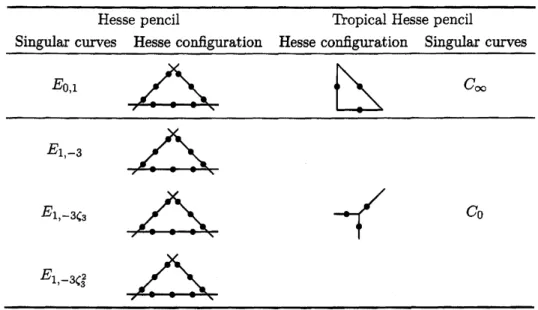
considerthe tropical counterpart of theHesseconfiguration. Rememberthat theHesse

configuration consists of the 9 inflection points$p0,p_{1},$$\cdots,p_{8}$ and the 12 inflectionslines, which

compose the singular members $E_{0,1},$ $E_{1,-3},$ $E_{1,-3\zeta_{3}}$, and$E_{1,-3\zeta_{3}^{2}}$ of the pencil (see table 1).

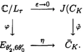
Fix$\tau$

as

in (23). We consider

a

map$\eta:E_{\theta_{2}’,6\theta_{0}’}arrow\overline{C}_{K}$

so

defined that the diagramcommute:

$\mathbb{C}/L_{\tau}arrow^{\text{\’{e}}arrow 0}J(C_{K})$

$\varphi\downarrow$ $\downarrow\overline{\varphi}$

$E_{\theta_{2}’,6\theta_{0}’}arrow^{\eta}$ $\overline{C}_{K}$

.

Theinflectionpoints of$E_{\theta_{2}’,6\theta_{\acute{0}}}$

are

mapped into the vertices of $\overline{C}_{K}$ by

$\eta$

as

follows $\eta:p_{0},$ $p_{1},$

$p_{2}^{\underline{\varphi^{-1}}}z_{20},$

$z_{21},$

$z_{22}arrow u_{2}V_{1}\epsilonarrow 0\underline{\tilde{\varphi}}$

$\eta:p_{3},$ $p_{4},$

$p_{5}^{\underline{\varphi^{-1}}}z_{00},$

$z_{01},$

$z_{02^{arrow u_{0}V_{2}}}^{\text{\’{e}}arrow 0\underline{\tilde{\varphi}}}$

$\eta:p_{6},$ $p_{7}$, $ps$

$\underline{\varphi^{-1}}z_{10},$

$z_{11},$

$z_{12^{arrow u_{1}V_{3}}}^{\epsilonarrow 0\underline{\tilde{\varphi}}}$

.

Thusthe tropical counterparts of theHesseconfiguration consistsof theverticesof$\overline{C}_{K}$ and the

lines passing through them. Moreover, the lines passing through the vertices should

compose

the singular members of the tropical Hesse pencil.

Table 2 showsthatthere exist two singular members$C_{0}$ and$C_{\infty}$ inthe tropical Hesse pencil.

The member$C_{0}$ isatripletropical lin$e$defined by (9). Each of the threepoints$V_{1},$ $V_{2}$, and $V_{3}$is

clearlyoneach ofthe three tentacles of$C_{0}$

.

On theother hand, the singular member$C_{\infty}$ is the

boundaryof$\mathbb{P}^{2,tr\varphi}$

defined by (5) (see (6)). Sincethepoints $V_{1},$ $V_{2}$, and $V_{3}$ arecontained inside

of$\mathbb{P}^{2,tr\varphi}$, it looks that they are not on $C_{\infty}$. However, noticing the linear equivalence relation $\sim$, which identifies all points on a tentacle, and the fact

a

tentacle to intersect

a

boundary of

$\mathbb{P}^{2,tr\varphi}$, wecanconclude

thatall thepoints$V_{1},$ $V_{2}$,and $V_{3}$ arecontained in$C_{\infty}$

.

Thusthe tropical

counterpart of the Hesse configurationconsists of three points and four lmes which $SatiS\mathfrak{h}r$the

following two conditions;

$\bullet$ each line passes throughat least

one

ofthe three points and

.

each point lies

on

two ofthe four lines.

Table 3: The correspondence between the Hesse configuration and its tropical counterpart.

Hessepencil TYopicalHesse pencil

Singular

curves

Hesse configuration Hesse configuration Singular

curves

$E_{0,1}$ $C_{\infty}$

$E_{1,-3}$

$E_{1,-3\zeta_{3}}$ $C_{0}$

$E_{1,-3\zeta_{3}^{2}}$

4.4

Ultradiscrete

elliptic functions

Now we construct the addition formula for the points onthe tropical Hesse curve viathe

ultra-discretizationof that for the Hesse cubic

curve3.

Forthispurpose, weintroduceelliptic functions

defined bythe ratios of the level-three theta functions:

$c(z):= \frac{\theta_{0}(z,\tau)}{\theta_{2}(z,\tau)}$ $s(z):= \frac{\theta_{1}(z,\tau)}{\theta_{2}(z,\tau)}$

.

It canbe easilychecked that the following holds

$c(z+1)=c(z)$ $c(z+\tau)=c(z)$

$s(z+1)=s(z)$ $s(z+\tau)=s(z)$

.

Therefore $c(z)$ and $s(z)$

are

elliptic functions which have the double periodicity withrespect to

the translations $zarrow z+1$ and $zarrow z+\tau$

.

In proposition 3, weshow that the followingholds for any $z=-a\tau\in d_{j}(j=1,2,3)$

$\lim_{\epsilonarrow 0}$elog$c(z)=\tilde{c}(u)$ and $\lim_{\epsilonarrow 0}\epsilon\log s(z)=\tilde{s}(u)$,

where$u=3Ka\in D_{j}$ and$\tau$ is assumed to be

as

in (23). Therefore, we call

$\tilde{c}$and $\tilde{s}$ultradiscrete

ellipticfunctions. Notethat $\tilde{c}(u)$ and$\tilde{s}(u)$ havesingle periodicity withrespect tothe translation

$uarrow u+3K$ (see figures 4(a) and $4(b)$).

The addition formulae for the elliptic functions $c(z)$ and $s(z)$

are

immediately follow $hom$

that forthe level-three thetafunctions (16), (17), and (18):

$c(z+w)= \frac{s(z)-c(z)^{2}c(w)s(w)}{c(z)c(w)^{2}-s(z)^{2}s(w)}$ (41a) $s(z+w)= \frac{c(z)s(z)s(w)^{2}-c(w)}{c(z)c(w)^{2}-s(z)^{2}s(w)}$ (41b)

$c(z+w)= \frac{c(z)s(z)c(w)^{2}-s(w)}{s(z)s(w)^{2}-c(z)^{2}c(w)}$ $s(z+w)= \frac{c(z)-s(z)^{2}c(w)s(w)}{s(z)s(w)^{2}-c(z)^{2}c(w)}$ (42a) (42b) $c(z+w)= \frac{c(z)s(w)^{2}-s(z)^{2}c(w)}{c(z)s(z)-c(w)s(w)}$ (43a) $s(z+w)= \frac{s(z)c(w)^{2}-c(z)^{2}s(w)}{c(z)s(z)-c(w)s(w)}$

.

(43b)

4.5

Addition

formula

Fix$\tau$

as

in (23). Assume $z$ and $w$ to be points

on

$l_{\epsilon}/\tau \mathbb{Z}$; thenwe

can

put them

as

follows $z= \frac{(1-i\xi_{\epsilon})u}{9K}$ and $w= \frac{(1-i\xi_{\epsilon})v}{9K}$,

where $u,$$v\in J(C_{K})$

.

Letus consider (41a). Byproposition 2,the ellipticfunctions $c$and $s$ arerealvalued forthis

choiceof$\tau$and $z,$ $w$. At first,

assume

$z,$ $w\in d_{1}$

.

Note thatthe followingholds (see (31))

$c(z),$$c(w)>0$, $s(z),$$s(w)<0$

.

Then wehave $s(z)=-|s(z)|$ $c(z)c(w)^{2}=|c(z)c(w)^{2}|$ $-c(z)^{2}c(w)s(w)=|c(z)^{2}c(w)s(w)|$ $-s(z)^{2}s(w)=|s(z)^{2}s(w)|$

.

It follows that the denominatoroftheright hand side of(4la) is alwayspositive, while thesign

of the numerator is indeterminate, i.e., it depends

on

the values of $z$ and $w$

.

The left hand

side of (41a) has the same sign

as

the numerator ofthe right hand side. Thus

we

obtain the

subtraction-free formof (4la)

$(|c(z)c(w)^{2}|+|s(z)^{2}s(w)|)|c(z+w)|+|s(z)|=|c(z)^{2}c(w)s(w)|$

if$|c(z)^{2}c(w)s(w)|>|s(z)|$

or

$(|c(z)c(w)^{2}|+|s(z)^{2}s(w)|)|c(z+w)|+|c(z)^{2}c(w)s(w)|=|s(z)|$

if $|c(z)^{2}c(w)s(w)|<|s(z)|$

.

Therefore, byproposition3, weobtain

$\tilde{c}(u+v)=\max(\tilde{s}(u), 2\tilde{c}(u)+\tilde{c}(v)+\tilde{s}(v))-\max(\tilde{c}(u)+2\tilde{c}(v), 2\tilde{s}(u)+\tilde{s}(v))$ (44)

except for $u,$$v$ satisfying $u+v=K^{4}$ in the limit $\epsilonarrow 0$

.

Since theboth hand sides of (44)

are

continuousfunctions, (44)holds

even

for$u,$$v$satisfying$u+v=K$

.

Noting(38),

we see

that (44)

holds for$u,$$v$such that both $(\tilde{c}(u),\tilde{s}(u))$ and $(\tilde{c}(v),\tilde{s}(v))$arein$E_{1}^{o}$, orequivalently, for_{$u,$ $v\in D_{1}$}

.

Next,

assume

$z\in d_{1}$ and $w\in d_{2}$

.

Thenwe have (see (31) and (32))

$c(z)>0$, $c(w),$ $s(z),$$s(w)<0$

.

The denominator of the right hand side of (4la) is always positive and the numerator is

al-ways negative. The left hand side of (41a) has the negative sign as well. Thus

we

obtain the

subtraction-free form

$(|c(z)c(w)^{2}|+|s(z)^{2}s(w)|)|c(z+w)|=|s(z)|+|c(z)^{2}c(w)s(w)|$

.

Taking the limit $\epsilonarrow 0$, we obtain (44) which holds for

$u,$$v$ such that $(\tilde{c}(u),\tilde{s}(u))\in E_{1}^{o}$ and

$(\tilde{c}(v),\tilde{s}(v))\in E_{2}^{o}$, orequivalently, for $u\in D_{1}$ and $v\in D_{2}$

.

Thus we observe that (44) is the candidate of the addition formula for the tropical Hesse

curve.

However, ifwe

assume

$z\in d_{1}$ and $w\in d_{3}$ then (44) does not hold. Actually, we have

(see (31) and (33))

$c(z),$_$s(w)>0$, $c(w),$$s(z)<0$

.

Inthis case, both the denominator and the numerator of (41a) have indeterminate sign. More

precisely, we have

$s(z)=-|s(z)|$

$c(z)c(w)^{2}=|c(z)c(w)^{2}|$

Thesubtraction-free form is

$-c(z)^{2}c(w)s(w)=|c(z)^{2}c(w)s(w)|$ $-s(z)^{2}s(w)=-|s(z)^{2}s(w)|$

.

$|c(z)c(w)^{2}||c(z+w)|+|s(z)|=|s(z)^{2}s(w)||c(z+w)|+|c(z)^{2}c(w)s(w)|$

or

$|c(z)c(w)^{2}||c(z+w)|+|c(z)^{2}c(w)s(w)|=|s(z)^{2}s(w)||c(z+w)|+|s(z)|$.

We then obtain the following in thelimit $\epsilonarrow 0$

$\max(\tilde{c}(u)+2\tilde{c}(v)+\tilde{c}(u+v),\tilde{s}(u))=\max(2\tilde{s}(u)+\tilde{s}(v)+\tilde{c}(u+v), 2\tilde{c}(u)+\tilde{c}(v)+\tilde{s}(v))$

.

(45)

In general, the valueof$\tilde{c}(u+v)$

can

notbedetermineduniquelyfromthoseof$\tilde{c}(u),\tilde{c}(v),\tilde{s}(u)$, and

$\tilde{s}(v)$ in terms of(45). Thusweseethat the

case

when$z\in d_{1}$and$w\in d_{3}$ theaddition formulafor

theultradiscreteellipticfunctionscannotbe reducedfrom (41a) through theultradiscretization.

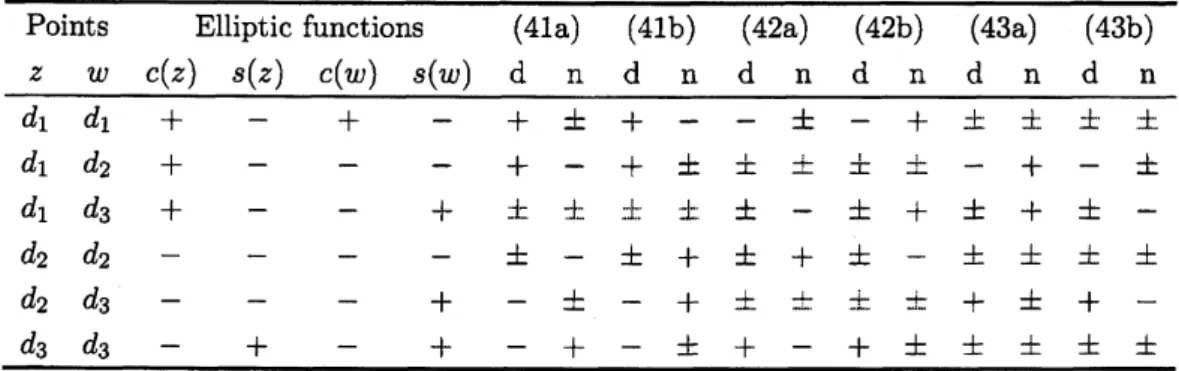
Table 4: The signs appearing in $(4la-43b)$

.

The denominator and the numerator of the right

hand sideofeach equation

are

denoted by $d$“ and $n$” respectively. The symbol $\pm$ stands for

indeterminate sign.

$\overline{Points}$

Elliptic functions(41a) (41b) (42a) (42b) (43a) (43b)

$\frac{zwc(z)s(z)c(w)s(w)dndndndndndn}{d_{1}d_{2}+---+-+\pm\pm\underline{arrow}\pm\pm-+-\cdot\pm d_{1}d_{1}+-+-+\pm+--\pm-+\downarrow-\pm\perp-\}}$

$d_{1}$ $d_{3}$ $+$ $-$ $-$ $+$ $:4_{\wedge}\wedge$ $\dotplus_{\sim}$ 4.$\cdot$

.$\cdot$ $\downarrow\sim$ $\pm$ _$-$ $\pm$ _$+$ $\pm$ $+$ $\pm$ _$-$

$d_{2}$ $d_{2}$ $-$ $-$ $-$ $-$ $\pm$ _$-$ $\pm$ _$+$ $\pm$ $+$ $\pm$ _$-$ $\pm$ $\pm$ $\pm$ $\pm$

$d_{2}$ $d_{3}$ _$-$ $-$ $-$ $+$ $-$ $\pm$ _{$-$ $+$} $\pm$ $\pm$ & $+$ $+$ $\pm$ _{$+$ $-$}

Thisfactsuggests that if both the denominator and thenumeratorhave indeterminate signs

then ordinary procedure of ultradiscretization

can

not be $applied^{5}$; otherwise,

we

can

apply it

to the additionformulae $(4la-43b)$

.

We summarize the signs of the equations $(4la-43b)$ for

thechoice of$z$ and$w$intable 4. From table4, weobserve thatwe canapplyordinary procedure

ofultradiscretization to $(4la-43b)$ except for the following

case

$z,$$w\in d_{j}$ $(j=1,2,3)$ $\Rightarrow$ (43a) and (43b)

$z\in d_{j},$$w\in d_{j+1}$ $(j=1,2,3)$ $\Rightarrow$ (42a) and (42b)

$z\in d_{j},$$w\in d_{j+2}$ $(j=1,2,3)$ $\Rightarrow$ (41a) and (41b),

where the subscripts

are

reduced modulo3.

Thus

we

have the following theorem.

Theorem 3 Assume $u\in\overline{D_{j}}$for

a

fixed$j=1,2,3$ , where $\overline{D_{j}}$is the closure of _{$D_{j}$}

.

Then the

ultradiscrete elliptic functions $\tilde{c}$ and $\tilde{s}$ satisfy thefollowing additionformulae

$\tilde{c}(u+v)=\max(\tilde{s}(u), 2\tilde{c}(u)+\tilde{c}(v)+\tilde{s}(v))-\max(\tilde{c}(u)+2\overline{c}(v), 2\tilde{s}(u)+\tilde{s}(v))$ (46a)

$\tilde{s}(u+v)=\max(\tilde{c}(u)+\tilde{s}(u)+2\tilde{s}(v),\tilde{c}(v))-\max(\tilde{c}(u)+2\tilde{c}(v), 2\tilde{s}(u)+\tilde{s}(v))$ , (46b)

ifand only if$v\in\overline{D_{j}\cup D_{j+1}}$,

or

$\tilde{c}(u+v)=\max(\tilde{c}(u)+\tilde{s}(u)+2\tilde{c}(v),\tilde{s}(v))-\max(\tilde{s}(u)+2\tilde{s}(v), 2\tilde{c}(u)+\tilde{c}(v))$ (47a)

$\tilde{s}(u+v)=\max(\tilde{c}(u), 2\tilde{s}(u)+\tilde{c}(v)+\tilde{s}(v))-\max(\tilde{s}(u)+2\tilde{s}(v), 2\tilde{c}(u)+\overline{c}(v))$, (47b)

ifand only if$v\in D_{j}\cup D_{j+2}$, or

$\tilde{c}(u+v)=\max(\tilde{c}(u)+2\tilde{s}(v), 2\tilde{s}(u)+\overline{c}(v))-\max(\tilde{c}(u)+\tilde{s}(u),\tilde{c}(v)+\tilde{s}(v))$ (48a)

$\tilde{s}(u+v)=\max(\tilde{s}(u)+2\tilde{c}(v), 2\tilde{c}(u)+\tilde{s}(v))-\max(\tilde{c}(u)+\tilde{s}(u),\tilde{c}(v)+\tilde{s}(v))$, (48b)

if and only if$v\in\overline{D_{j+1}\cup D_{j+2}}$, where the subscripts

are

reduced modulo 3.

(Proof) The “ _if“ _part

can

_{be shown by using such limiting procedure}

as

_demonstrated

above. For the boundary values ofthe closures, $u_{0},$ $u_{1}$, and $u_{2}$, the formulae

can

be shown by

direct calculation. By substituting appropriate values, say$u\in D_{1}$ and $v\in D_{3}$, into (46a), then

we

find that the equationdoesnot hold. In

a

similar manner,

we

can

prove the “_{only if}“ _part

for all

cases.

$\blacksquare$

Itimmediately follows theadditionformula for the pointson thetropical Hesse

curve

$C_{K}$

.

Corollary 1 Let $P=(X, Y)$ be a point on

an

edge $E_{j}$ of the tropical Hesse

curve

$C_{K}$ for a

fixed$j=1,2,3$

.

Then the point $P|dQ=(x\omega X’, Y\cup Y’)$ _{is given bythe following addition}

formulae

$X^{\ovalbox{\tt\small REJECT}} \theta X’=\max(Y,$$2X+X’+ Y’)-\max(X+2X’,$$2Y+Y’)$ (49a)

$Y \omega Y’=\max(X+Y+2Y’,$$X’)- \max(X+2X’,$$2Y+Y’)$ , (49b)

ifand only if$Q=(X’, Y’)\in E_{j}\cup E_{j+1}$, or

$X \cup X’=\max(X+Y+2X’, Y^{l})-\max(Y+2Y’, 2X+X’)$ (50a)

$Y \omega Y’=\max(X, 2Y+X’+Y’)-\max(Y+2Y’, 2X+X’)$, (50b)

if and only if$Q\in E_{j}\cup E_{j+2}$,

or

$X \cup X’=\max(X+2Y’, 2Y+X’)-\max(X+Y, X’+Y’)$ (51a)

$Y\oplus Y’=\max(Y+2X’, 2X+Y’)-\max(X+Y,X’+Y’)$, (51b)

ifandonly if$Q\in E_{j+1}\cup E_{j+2}$, where the subscripts

are

reduced modulo 3.

5

Conclusion

We give the addition formula $(49a-5lb)$ _{for the tropical Hesse pencil via the ultradiscretization}

ofthat $(12a-14c)$ for thelevel-threethetafunctions. Each pair $(49a, 49b),$ $(50a, 50b)$, or $(51a$, $51b)$ holdsexcept for

an

edge of the curve, while those _{$(12a-12c),$ $(13a-13c)$,} or _$(14a-14c)$

holds except forthreeof the9zerosofthe theta functions on$\mathbb{C}/L_{\tau}$

.

In the tropicalcase, two of

thethreepairs

are

essentially the

same

whereboth of them

are

defined. Therefore, the addition

formulauniquelydetermines the additivegroup structure ofthe tropicalHesse pencil in analogy

to theoriginal (non-tropical) case.

In [3], we construct the solvable chaotic dynamical system via the duplication formula for

the tropical Hesse pencil. The ultradiscrete QRT map $P=(X, Y)\mapsto\overline{P}=P$_ffl$T=(X, Y)–$

can

similarly be constructed by using the addition $\Theta$ of the tropical Hesse pencil. For example, if

wechoose $V_{3}$

as

$T$then, by using corollary 1,

we

obtain the linear map:

$\overline{X}=-X+Y$

$\overline{Y}=-Y+\overline{X}$

.

Thismap is periodic with period three foranyinitialvalue because$V_{3}$ isthethree-torsionpoint

of the pencil. This reflects the correspondence $\eta$ : $p_{6},p_{7},p_{8}\mapsto V_{3}$ , where $p_{6},$ $p_{7}$, and $p_{8}$

are

thethree-torsion points of the Hesse pencil. Thuswe

can

construct bothchaotic and integrable

dynamical systems by using the group structureofthe tropicalHesse pencil.

Acknowledgment

The author would like to express his sincere thanks to Professor Kenji Kajiwara for fruitful

discussion. This work

was

partially supported by grants-in-aid for scientific research, Japan

society for the promotion ofscience (JSPS) 19740086 and22740100.

References

[1] Artebani M and Dolgachev I “The Hesse pencil of plane cubic curves” Preprint

arXiv:math$/0611590v3$ (2006)

[2] Isojima S, MurataM, Nobe A and Satsuma J “Soliton-antisoliton collision in the

ultradis-crete modified KdVequation” Phys. Lett. A 357 (2006) 31-35

[3] Kajiwara K, Kaneko M, Nobe A and Tsuda T ”Ultradiscretization of a solvable

two-dimensional chaotic map associatedwith theHessecubic curve” KyushuJ. Math. 63 (2009)

315-338

[4] Kajiwara K, Nobe A and TsudaT ”Ultradiscretization of solvable one-dimensional chaotic

maps” J. Phys. A: Math. Theor. 41 (2008) 395202

[5] MikhalkinGandZharkovI “Tropicalcurves, theirJacobians andtheta functions” Preprint

$arXiv:math/0612267vl$ (2006)

[6] Nakamura I “Plane cubic curves–from Hesse to Mumford-,‘ _{Sugaku June (2001) 17-34}

(in Japanese)

[7] Nobe A “Ultradiscrete QRT maps and tropical elliptic curves” J. Phys. A: Math. Theor.

[8] Shaub HC and Schoonmaker HE “The Hessian configuration and its relation

to

the

group

of order 216” Am. Math. Mon. 38 (1931)

38&393

[9] VigelandMD “Thegrouplawon

a

tropical elliptic curve” Preprint$arXiv:math/04114S5vl$