〈寄稿論文〉A Model of Class Identification :
Generalization of the Fararo-Kosaka Model
using Lyapounov’s Central Limit Theorem
journal or
publication title
社会学部紀要
number
114
page range
23-35
year
2012-03-15
URL
http://hdl.handle.net/10236/9004
1. Introduction: Fararo-Kosaka model of class identification
In this paper, we explore a mechanism for generating a class identification process. We use the con-cept of “class identification” in the following sense. In empirical studies based on social surveys, class identification is often defined operationally as an answer to the question ‘If we were to divide the en-tire society into several levels, which level would you say you belong to?’ We treat the respondents’ answer to this question as their self-location in society. For example, in a Social Stratification and Mo-bility survey, the response categories for the question of class identification are ‘upper, upper middle, lower middle, upper lower, and lower lower.’ Empirical studies of class identification mainly focus on specifying its social and economic determinants. Such studies have demonstrated historical changes af-fecting social status such as household and individual income, education, occupation, gender, and age based on class identification (Shirahase 2010). These empirical studies provide basic assumptions for making an abstract model.
There are many empirical studies of class identification based on statistical analysis whereas few theoretical studies attempt to explain a mechanism for generating a class identification process. For-malization studies are likely to explain a mechanism by making a model rather than describing histori-cal changes in the determinants of class identification. The model of the image of stratification formal-ized by Fararo and Kosaka is one of the most significant studies in the field of social stratification be-cause the model attempts to explain how individual actors located in the structure of any given social system acquire a stable image of the structure, which varies with location, and how the actors locate themselves within their structural image. The Fararo-Kosaka model (hereafter, FK model) explicitly formalized the process whereby people compare their social status with others to build an image of so-cial stratification where they could locate their class identity based on a subjective image of stratifica-tion. The FK model has many interesting implications and it successfully explains the magnification of middle class identification (Kosaka 2006; Fararo and Kosaka 2003). Many studies have attempted to develop the FK model further (Shirakura and Yosano 1991; Yosano 1996; Ishida 2003, 2005; Karpin-ski 2009; Maeda 2011).
The FK model assumes that each dimension of social status, such as education, income, and occu-pation, has an internal rank and that the ranges of ranks are equal among dimensions. Suppose that r1,
r2, ..., rnare the maximum values of numbers in the ranks of each dimension. For example r1 is the 〈寄稿論文〉
A Model of Class Identification:
*Generalization of the Fararo-Kosaka Model using Lyapounov’s Central Limit Theorem
Hiroshi HAMADA
**─────────────────────────────────────────────────────
*
Key Words: class identification, Fararo-Kosaka model, central limit theorem
**Associate Professor, Tohoku University
maximum value in ranks of the first dimension, r2is that of the second dimension, and so on. The FK model assumes that r1=r2=・・・=rn for all dimensions. This assumption implies that if education is
measured using five ranks, then other dimension of social status, for example income, should be also divided into five categories. The number of ranks in each dimension directly has an effect on the posi-tion of self-locaposi-tion in a society. Therefore, the assumpposi-tion of rank homogeneity may be too strong. However, few studies have explored the implications when the rank homogeneity assumption is re-laxed from both theoretical and empirical perspectives. In this paper, we generalize the rank homoge-neity assumption and show that the empirical validity of the model will be improved by this generali-zation. In other words, we attempt to generalize the FK model theoretically and empirically.
The remainder of this paper is organized as follows. In section 2, we apply Lyapounov’s central limit theorem to the FK model to generalize the condition of the marginal distribution of social status and we prove that the main proposition of the FK model still holds when each dimension of social status obeys a non-identical discrete uniform distribution with different ranges. In section 3, we further generalize the FK model by applying the central limit theorem and we show that the distribution of standardized class identification asymptotically obeys the normal distribution, if each distribution of the dimensions has a finite mean and variance, and the maximum value of ranks and the dimensions are independent of each other. In section 4, we test the empirical validity of the generalized FK model by checking the correlation between the theoretical predictions of class identification from the FK model and observed data of class identification in an SSM survey. In section 5, we summarize the re-sults of the mathematical analysis and empirical test.
2. Non-identical discrete uniform distribution model
Definition (a set of profiles of social status). Social stratification consists of n dimensions and each
dimension has an internal rank. The rank in each dimension is given by a natural number. For the ith dimension, {1, 2, ..., ri} is as a set of ranks. riindicates the highest rank of the ith dimension. A set of
profiles of social status is expressed as direct products of the sets of ranks. We call this S and it is ex-plicitly given by
S={1, 2, ..., r1}×{1, 2, ..., r2}×・・・×{1, 2, ..., rn}.
Individual social status profiles are defined as a point (x1, x2, ..., xn)∈S . Generally, the ranges of ranks
for dimensions are different from each other. We allow cases such as ri≠rj. Conversely, if the special
condition r1=r2=・・・=rn is satisfied, the definition of a set of social status profiles corresponds to
that of the FK model.
For example, suppose there are two dimensions such as education and wealth. The first dimension has three ranks (low, middle, and high) while the second dimension has two ranks (poor and rich). A set of profile of social status is then,
S={1, 2, 3}×{1, 2}={(1, 1), (1, 2), (2, 1), (2, 2), (3, 1), (3, 2)}. Individual social status profiles are (1, 1), (1, 2), (2, 1), (2, 2), (3, 1) and (3, 2).
The FK model assumes that actors are stratified along a number of salient dimensions and that the
dimensions of stratification are themselves ordered relative to their importance. Therefore, it is possi-ble to combine positions occupied by the actors in each dimension to arrive at a single ordering of the members of the system. In the FK model, the ordering is defined using the lexicographic order (Fararo and Kosaka 2003; Karpinski 2009). According to this rule, if person p occupies a higher position than person o in the most socially significant dimension, then p is higher than o in the overall ordering, re-gardless of the positions they occupy in the remaining dimensions of stratification. Thus, if p and o are status-equals with respect to the first dimension, but o is higher along the second one, then o is also higher in the overall ordering of positions. For example, suppose that there is a society with struc-ture S={1, 2, 3}×{1, 2} and the first dimension is more important than the second dimension. Suppose that the magnitude of numbers corresponds to the order of rank (larger number indicates high status). The lexicographic order determines the rank of profiles as follows; (3, 2)! (3, 1) ! (2, 2) ! (2, 1)! (1, 2) ! (1, 1).
Corollary 1 (rank of class identification). Suppose that the focal actor has profile (x1, x2, ..., xn). The
rank of self-location in its image of stratification is
n
!
i=1xi−(n−1).
This equation indicates the rank of class identification from the bottom.
Proof. The proof of this corollary is almost trivial because we can use the result of a previous study
(Kosaka 2006). Let (x1, x2, ..., xn) be the profile of the focal actor. In the first dimension, the number
of cases where the ranks of other are smaller than the focal actor’s rank is x1−1. The number of cases where the ranks of others are equal to the focal actor’s rank in the first dimension and the ranks of others are smaller than the focal actor’s rank in second dimension are x2−1. Similarly, the number of cases where the ranks of others are equal to the focal actor’s rank from first dimension to n−1th di-mension and ranks of others are smaller than the focal actor’s rank in the nth didi-mension are xn−1.
Therefore, all possible patterns where the ranks of other profiles are below the focal actor’s profile is
!n
i=1(xi−1). The focal actor’s subjective class identification from the bottom is !ni=1(xi−1). We
ob-tain
!n
i=1(xi−1)+1=!ni=1xi−n+1=!ni=1xi−(n−1)
Proposition 1 (probability function of class identification). Suppose that the rank of each dimension is
represented using non-identical and independent discrete uniform distributions. The probability that an actor’s class identification becomes x is
Pr{X=x}=
(
nΠ
i=1ri)
−1 βx whereβx=#{y=(y1, y2, ..., yn) | y∈S, n
!
i=1yi−(n−1)=x}.
2.0 1.5 1.0 0.5 6 5 4 3 2 1 30 25 20 15 10 5 8×2 8×2×3 8×2×3×5
In the above equation #A indicates the number of elements in set A.
Proof. Class identification of profile y=(y1, y2, ..., yn) in S is n
!
i=1yi−(n−1). Let this value be x. There are several profiles whose class identification becomes x. The number of patterns can be repre-sented by
#{y=(y1, y2, ..., yn) | y∈S , n
!
i=1yi−(n−1)=x}. (1)
Based on the assumption of the independence of random variables, for all y=(y1, y2, ..., yn), we have
Pr{(Y1=y1)∩(Y2=y2)∩・・・∩(Yn=yn)}=Pr{Y1=y1} Pr{Y2=y2}・・・Pr{Yn=yn}=1
r1 1
r2・・・ 1
rn.
The number of patterns where the class identification becomes x is expressed by (1), and each pattern is mutually exclusive. Thus,
Pr{X=x}=
(
nΠ
i=1r i)
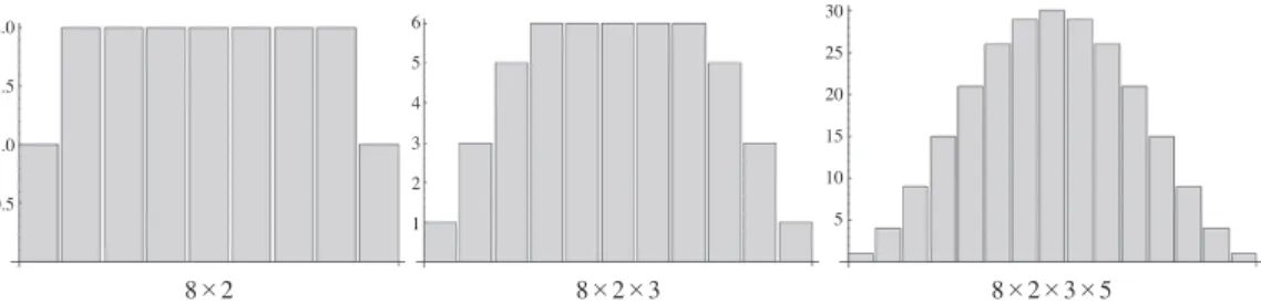
−1 βx.Figure 1 shows the distributions of class identification generated by the probability function in Proposition 1. In Figure 1, 8×2 means that the number of ranks in the first dimension is 8 and the number of ranks in second dimension is 2. Similarly, 8×2×3 means that 8 is the number of ranks in first dimension, 2 is that in the second dimension, and 3 is that in the third dimension.
In terms of probability theory, we then have to specify the distribution of class identification de-rived from the FK model where the range of ranks for each dimension is different from each other.
Let, Xi be a discrete random variable and 1, 2, ..., ri be its values. We can define a new random
variable Snby composing n random variables as follows.
Sn= n
!
i=1Xi−(n−1)
The class identification distribution is specified by identifying a probability function Pr{Sn=j}=f (j) .
Yosano (1996) proved the very important proposition that the class identification distribution obeys the normal distribution when a random variable in each dimension independently obeys an identical uniform distribution. The rank homogeneity assumption, i.e., the identical distribution assumption,
Figure 1 Distribution of class identification. Numbers at the bottom of the graph indicate the rank of each
dimension. The distribution is computed given the condition that there is only one person in each profile.
means that education, income, and occupation are subject to identical distribution with the same range. We know that the formalization approach often uses such strong assumptions to simplify a model while the strong assumption itself has no problem. However, if we can relax the strong assumptions without any loss of generality, this will expand the universality of the theory. Moreover, we can ex-pect to improve empirical validity of the model by this generalization.
We will show that, even when a random variable in each dimension obeys a non-identical and inde-pendent uniform distribution, the class identification also obeys a normal distribution. In order to test this proposition, we use the following general theorem of the probability theory.
Theorem 2 (Lyapounov’s central limit theorem). Suppose that {Xj} is a sequence of independent
random variables and each random variable has a mean of E (Xj)=μj and a variance V (Xj)=σj2.
Suppose that Bn=
"
σ12+σ22+・・・+σn2and for someδ >0, condition
lim n→∞ 1 Bn2+δ n ! j=1E [ |Xj−μj| 2+δ]=0 holds. Then, Yn=((X1−μ1)+(X2−μ2)+・・・+(Xn−μn)) /Bn
obeys a standard normal distribution N (0, 1). Proof. Details are given in Billingsley (1986).
Note that, in Theorem 2 the components of the random variable sequence {Xj} are not necessarily
identical. It is enough that the mean and variance hold the condition of 2+δ th order moment. We re-fer to this as Lyapounov’s condition.
Proposition 3. Suppose that a set of social status profiles is expressed as the direct product of sets of
ranks, S={1, 2, ..., r1}×{1, 2, ..., r2}×・・・×{1, 2, ..., rn}. When a random variable in each
di-mension obeys a non-identical and independent uniform distribution, the standardized class identifica-tion distribuidentifica-tion obeys a standard normal distribuidentifica-tion N (0, 1) if n is sufficiently large.
Proof. Let Xjbe a random variable in a discrete uniform distribution of the jth dimension. The values
of Xjare 1, 2, ..., rj. Let K>0 be the maximum number of ranks in all dimension. Thus, for all j,
max
j (rj)=K . For all j, an absolute third order moment of Xjsatisfies E [ |Xj−μj|3]= rj ! i=1|i−μj| 3 1 rj= rj ! i=1|i−μj| | i−μj| 2 1 rj< rj ! i=1K |i−μj| 2 1 rj=Kσ j2.
We use the following relation |i−μj|<K for all i (i=1, 2, ..., rj). Based on the inequality with
re-spect to an absolute third order moment, we have 1 Bn3 n ! j=1E [ |Xj−μj| 3]< 1 Bn3 n ! j=1Kσj 2 and March 2012 ― 27 ―
lim n→∞ 1 Bn3 n ! j=1Kσj 2= lim n→∞ KBn2 Bn3 = limn→∞ K Bn=0 .
Since the limit of the sum of absolute values is not negative, lim n→∞ 1 Bn3 n ! j=1E [ |Xj−μj| 3]
should not be negative. Because∀n, an<bn⇒ lim
n→∞an!limn→∞bn, we obtain 0!limn→∞B1 n3 n ! j=1E [ |Xj−μj| 3 ]!lim n→∞ 1 Bn3 n ! j=1Kσj 2=0 ⇒ lim n→∞ 1 Bn3 n ! j=1E [ |Xj−μj| 3 ]=0 This implies that, forδ =1, Lyapounov’s condition is satisfied. Therefore,
Yn=((X1−μ1)+(X2−μ2)+・・・+(Xn−μn)) /Bn
obeys a standard normal distribution N (0, 1). As shown, the class identification is given by
Y=X1+X2+・・・+Xn−(n−1) .
If we standardize Y as Yn={Y +(n−1)− n
!
i=1μi} /Bn, Ynobeys a standard normal distribution N (0, 1) based on the central limit theorem.
Using the following corollary, we can specify the class identification distribution.
Corollary 2. When a random variable in each dimension independently obeys a non-identical uniform
distribution, the non-standardized class identification distribution obeys an approximately normal dis-tribution with a mean (
n ! j=1μj)−(n−1) and a variance n ! j=1 rj2 12, if n is sufficiently large. Proof. From Yn=((X1−μ1)+(X2−μ2)+・・・+(Xn−μn)) / Bn, X1+X2+・・・+Xn=BnYn+ n ! j=1μj. Because Ynobeys a standard normal distribution, X1+X2+・・・+Xnobeys a normal distribution. When
Xj obeys a discrete uniform distribution with the range [1, rj], its variance is V (Xj)=rj2/12.
There-fore, the variance of X1+X2+・・・+Xnwill be the variance of Yntimes Bn2.
1・Bn2=σ12+σ22+・・・+σn2= n ! j=1 rj2 12. Therefore, X1+X2+・・・+Xn obeys a normal distribution,
N
(
( n ! j=1μj), n ! j=1 rj2 12)
.Subtracting constant, X1+X2+・・・+Xn−(n−1) obeys a normal distribution,
N
(
( n ! j=1μj)−(n−1), n ! j=1 rj2 12)
. ― 28 ― 社 会 学 部 紀 要 第114号0.5 0.4 0.3 0.2 0.1 2 4 6 8 10 12 14 16
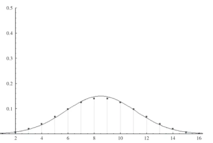
Figure 2 shows an example of this corollary.
3. General model
Note that Proposition 3 and Corollary 2 hold only when a random variable in each dimension inde-pendently obeys a uniform distribution. This condition is not usually satisfied in the real world. How-ever, when Lyapounov’s condition holds we obtain a normal distribution as a class identity distribu-tion. Thus, we do not have to assume a uniform distribution in order to derive a normal class identity distribution from the FK model.
Proposition 4. Suppose that a set of social status profiles is expressed as a direct product of sets of
ranks, S={1, 2, ..., r1}×{1, 2, ..., r2}×・・・×{1, 2, ..., rn}. When random variables from each
di-mension are independent of each other, they have a finite mean E (Xj)=μjand a variance V (Xj)=σj2,
respectively. If lim
n→∞σ1 2+σ
22+・・・+σn2=∞ holds, then the standardized class identification
distribu-tion obeys a standard normal distribudistribu-tion N (0, 1), if n is sufficiently large.
Proof. Let Xjbe a random variable in the ith dimension. The values of Xjare 1, 2, ..., rj. Let K>0 be
a maximum number of ranks in all dimension and fj(x) be a probability function of Xj. For all j , the
absolute third order moment of Xjsatisfies
E [ |Xj−μj|3]= rj ! i=1|i−μj| 3 fj(i)! rj ! i=1K |i−μj| 2 fj(i)=Kσj2.
Based on a similar logic to the proof of Proposition 3, we have
───────────────────────────────────────────────────── 1)More accurately, the line indicates the plot of a probability density function for a normal distribution with the mean
(
!5j=1μj
)
−4 and the variance(
!5
j=1rj2/12
)
.Figure 2 Plot of a discrete probability function and a continuous probability density
function of a class identification distribution, which is theoretically specified where
r1=3, r2=4, r3=2, r4=6, r5=5. Points on the graph correspond to the values of the probability function while the curved line corresponds to a plot of the probability
den-sity function1).
lim n→∞ 1 Bn3 n ! j=1E [ |Xj−μj| 3]=0
This implies that, for δ =1, Lyapounov’s condition is satisfied. When we standardize the class identi-fication by Yn={Y +(n−1)−
n
!
i=1μi}/ Bn, Yn obeys a standard normal distribution N (0, 1) based on the central limit theorem.
Proposition 4 has a very strong and general implication for the FK model. Whenever each social status dimension has a finite mean and variance (this is a quite natural assumption), the class identification distribution obeys a normal distribution if the number of dimensions is sufficiently large. This is very important because Proposition 4 allows us to assume any empirical distribution for each dimension of social stratification. As Figure 2 shows, four or five dimensions are enough for approximation by a normal distribution, although the number of dimensions n should be infinitely large in theory. It is im-portant for us to reconsider the assumption of the independence of random variables in dimensions. It is well known that the dimensions of social status are correlated with each other. For example, educa-tion and income have a positive correlaeduca-tion while occupaeduca-tional prestige score and income also have a positive correlation. These correlations may affect the fitness of data.
4. Empirical validity of the generalized FK model
In this section, we test the empirical validity of the FK model based on the results from the previ-ous section. We used Social Stratification and Mobility Survey (SSM) data from 1955 to 2005. For time-series comparisons, we used only the male date set. The procedure of the empirical test was as follows.
First, we defined the range of ranks in each dimension. Dimensions such as education are easy to fix the number of ranks because it is naturally divided into finite categories. In order to compare data in time-series, we used three categories for education. The codes were: 1: elementary and junior high school level; 2: high school level; and 3: university and higher level. In contrast, it is not easy to fix the number of ranks for dimensions such as income and occupation because they do not have natural distinctive points for categorization. Therefore, we used different numbers of ranks experimentally. According to previous research, we know that people often view occupation as four or five categories (Shiotani 2010). We used 3 to 8 ranks for occupation. The ranks are computed based on the occupa-tional prestige score of the SSM survey. Incomes were measured using various scales in each survey period. For example, a 10 point scale was used in 1955, a continuous scale in 1965, and a 30 point scale in the 1995 and 2005 surveys. Therefore, we used 5 to 30 ranks for dividing the income range.
Second, the theoretical class identification prediction was computed as follows. Three independent variables were used, i.e., family income, education level, and occupation prestige score. For example, if a subject i has a profile such as (family income 10, education level 2, prestige score 5), we assume that his theoretical class identification is 10+2+5−2=15 based on Corollary 1. We computed all theoretical prediction of class identification for all possible patterns of combinations of ranks, i.e., sample size×6 (patterns of occupation rank)×26 (patterns of income rank).
Third, we computed the correlation coefficient between the theoretical class identification prediction from the generalized FK model and the observed class identification data collected by the SSM
veys. As mentioned earlier in this paper, the SSM survey asks respondents to locate their subjective class identification into five categories: Upper, Upper Middle, Lower Middle, Upper Lower, and Lower Lower.
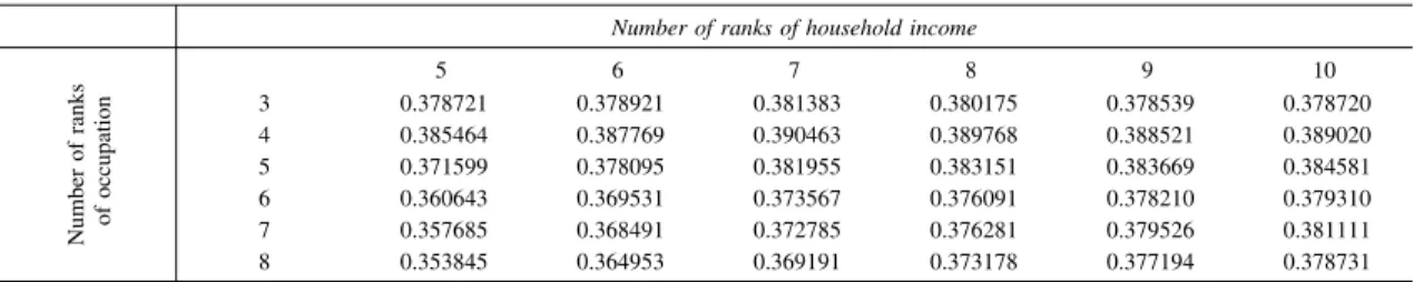
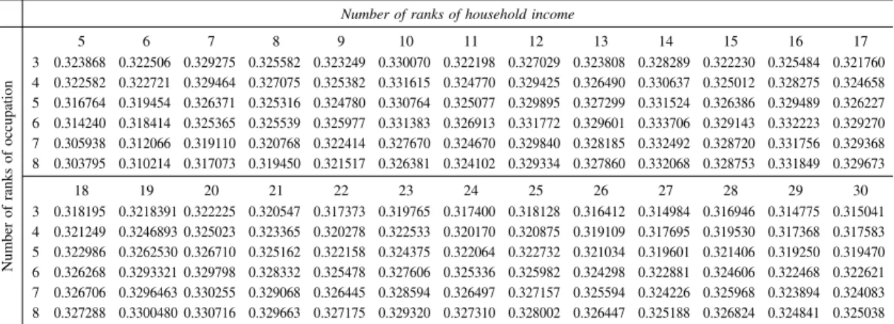
In the following tables, the numbers in each cell indicate the correlation coefficient between the ob-served class identification from data and the theoretical prediction of the model. Rows correspond to number of rank divisions for occupational prestige while columns correspond to the number of rank divisions of household income.
Table 1 Correlation coefficients for the theoretical class identification predictions of the model and the observed data
from the 1955 SSM (males).
Number of ranks of household income
5 6 7 8 9 10 3 4 5 6 7 8 0.378721 0.385464 0.371599 0.360643 0.357685 0.353845 0.378921 0.387769 0.378095 0.369531 0.368491 0.364953 0.381383 0.390463 0.381955 0.373567 0.372785 0.369191 0.380175 0.389768 0.383151 0.376091 0.376281 0.373178 0.378539 0.388521 0.383669 0.378210 0.379526 0.377194 0.378720 0.389020 0.384581 0.379310 0.381111 0.378731
Table 2 Correlation coefficients for the theoretical class identification predictions of the model and the observed data
from the 1965 SSM (males).
Number of ranks of household income
5 6 7 8 9 10 11 12 13 14 15 16 17 3 4 5 6 7 8 0.347073 0.340050 0.328911 0.322503 0.318410 0.319416 0.351024 0.346461 0.337287 0.332087 0.328622 0.329639 0.353398 0.350294 0.342521 0.338296 0.335300 0.336516 0.355487 0.353770 0.347140 0.343959 0.341517 0.342946 0.355041 0.354005 0.348417 0.345831 0.343838 0.345401 0.355746 0.355633 0.350959 0.349197 0.347455 0.349369 0.353729 0.354165 0.350425 0.349325 0.348152 0.350307 0.351272 0.352545 0.349717 0.349568 0.348873 0.351420 0.351797 0.353258 0.350751 0.350841 0.350379 0.352948 0.349756 0.351624 0.349743 0.350399 0.350173 0.353051 0.349041 0.351004 0.349541 0.350478 0.350524 0.353447 0.349078 0.351304 0.350093 0.351404 0.351618 0.354672 0.350913 0.353183 0.352203 0.353592 0.353881 0.356951 18 19 20 21 22 23 24 25 26 27 28 29 30 3 4 5 6 7 8 0.347560 0.349988 0.349253 0.350921 0.351365 0.354595 0.347238 0.349775 0.349245 0.351122 0.351715 0.354985 0.347147 0.349652 0.349285 0.351246 0.351863 0.355120 0.346351 0.348902 0.348684 0.350754 0.351487 0.354783 0.344636 0.347204 0.347166 0.349348 0.350159 0.353488 0.343792 0.346381 0.346458 0.348763 0.349701 0.353021 0.342751 0.345406 0.345537 0.347908 0.348840 0.352228 0.342247 0.344817 0.345070 0.347436 0.348436 0.351754 0.342837 0.345425 0.345671 0.348065 0.349033 0.352345 0.342134 0.344740 0.345064 0.347505 0.348497 0.351821 0.341054 0.343612 0.344038 0.346511 0.347550 0.350844 0.340449 0.342996 0.343462 0.345950 0.347029 0.350300 0.340167 0.342706 0.343172 0.345661 0.346699 0.349965
Table 3 Correlation coefficients for the theoretical class identification predictions of the model and the observed data
from 1975 SSM (males).
Number of ranks of household income
5 6 7 8 9 10 11 12 13 14 15 16 17 3 4 5 6 7 8 0.216181 0.202164 0.203985 0.198935 0.194131 0.192511 0.222304 0.211051 0.212898 0.208440 0.204009 0.202455 0.226590 0.216679 0.218701 0.214583 0.210414 0.208943 0.223880 0.215976 0.218397 0.215158 0.211697 0.210780 0.223649 0.217569 0.220176 0.217734 0.215054 0.214577 0.224583 0.218137 0.220725 0.218039 0.215170 0.214681 0.224967 0.219790 0.222462 0.220379 0.218078 0.217957 0.224365 0.220253 0.222984 0.221445 0.219713 0.219927 0.223691 0.220055 0.222835 0.221550 0.220042 0.220449 0.227413 0.223600 0.226261 0.224801 0.223177 0.223472 0.224773 0.221602 0.224356 0.223289 0.222030 0.222634 0.222517 0.219941 0.222723 0.222012 0.221132 0.221981 0.222795 0.220492 0.223262 0.222705 0.221993 0.222965 18 19 20 21 22 23 24 25 26 27 28 29 30 3 4 5 6 7 8 0.220109 0.218223 0.221016 0.220721 0.220285 0.221449 0.221673 0.219809 0.222509 0.222178 0.221749 0.222903 0.221153 0.219392 0.222125 0.221870 0.221488 0.222722 0.220678 0.219206 0.221867 0.221771 0.221584 0.222902 0.220179 0.218934 0.221525 0.221558 0.221513 0.222906 0.219516 0.218353 0.220924 0.220994 0.221010 0.222444 0.21986 0.218782 0.221304 0.221417 0.221483 0.222938 0.219097 0.218138 0.220640 0.220821 0.220959 0.222453 0.218839 0.218014 0.220442 0.220694 0.220913 0.222434 0.219449 0.218670 0.221059 0.221327 0.221572 0.223087 0.219490 0.218718 0.221092 0.221350 0.221589 0.223119 0.219122 0.218457 0.220764 0.221077 0.221380 0.222924 0.217932 0.217334 0.219634 0.219990 0.220339 0.221911 Number of ranks of occupat io n Number of ranks of occupat io n Number of ranks of occupat io n March 2012 ― 31 ―
Table 4 Correlation coefficients for the theoretical class identification predictions of the model and the observed data from the 1985 SSM (males).
Number of ranks of household income
5 6 7 8 9 10 11 12 13 14 15 16 17 3 4 5 6 7 8 0.249602 0.243616 0.249107 0.232579 0.229497 0.215211 0.262136 0.257325 0.261771 0.246834 0.243604 0.229955 0.265811 0.262176 0.266199 0.252781 0.249875 0.237208 0.275087 0.271820 0.275333 0.262366 0.259238 0.246793 0.274646 0.272488 0.275937 0.264825 0.262361 0.251178 0.279240 0.277546 0.280699 0.270369 0.268082 0.257452 0.279301 0.278230 0.281357 0.272125 0.270275 0.260513 0.278391 0.277922 0.281097 0.272982 0.271611 0.262809 0.279923 0.279744 0.282811 0.275307 0.274139 0.265844 0.279364 0.279524 0.282638 0.275938 0.275155 0.267619 0.283050 0.283321 0.286229 0.279762 0.279000 0.271654 0.284976 0.285356 0.288128 0.282194 0.281581 0.274765 0.283089 0.283720 0.286533 0.281256 0.280971 0.274824 18 19 20 21 22 23 24 25 26 27 28 29 30 3 4 5 6 7 8 0.281070 0.281893 0.284740 0.279906 0.279839 0.274142 0.282188 0.283098 0.285880 0.281384 0.281435 0.276106 0.283885 0.284822 0.287468 0.283262 0.283407 0.278351 0.281900 0.282975 0.285633 0.281867 0.282231 0.277660 0.281656 0.282793 0.285419 0.281863 0.282318 0.277963 0.283318 0.284469 0.287021 0.283606 0.284048 0.279878 0.283467 0.284626 0.287113 0.283938 0.284482 0.280544 0.283977 0.285193 0.287634 0.284709 0.285339 0.281669 0.282972 0.284208 0.286602 0.283754 0.284402 0.280840 0.282733 0.283975 0.286332 0.283704 0.284426 0.281107 0.281051 0.282345 0.284704 0.282306 0.283129 0.280081 0.280985 0.282279 0.284567 0.282262 0.283104 0.280156 0.283165 0.284457 0.286694 0.284470 0.285308 0.282473
Table 5 Correlation coefficients for the theoretical class identification predictions of the model and the observed data
from the 1995 SSM (males).
Number of ranks of household income
5 6 7 8 9 10 11 12 13 14 15 16 17 3 4 5 6 7 8 0.323868 0.322582 0.316764 0.314240 0.305938 0.303795 0.322506 0.322721 0.319454 0.318414 0.312066 0.310214 0.329275 0.329464 0.326371 0.325365 0.319110 0.317073 0.325582 0.327075 0.325316 0.325539 0.320768 0.319450 0.323249 0.325382 0.324780 0.325977 0.322414 0.321517 0.330070 0.331615 0.330764 0.331383 0.327670 0.326381 0.322198 0.324770 0.325077 0.326913 0.324670 0.324102 0.327029 0.329425 0.329895 0.331772 0.329840 0.329334 0.323808 0.326490 0.327299 0.329601 0.328185 0.327860 0.328289 0.330637 0.331524 0.333706 0.332492 0.332068 0.322230 0.325012 0.326386 0.329143 0.328720 0.328753 0.325484 0.328275 0.329489 0.332223 0.331756 0.331849 0.321760 0.324658 0.326227 0.329270 0.329368 0.329673 18 19 20 21 22 23 24 25 26 27 28 29 30 3 4 5 6 7 8 0.318195 0.321249 0.322986 0.326268 0.326706 0.327288 0.3218391 0.3246893 0.3262530 0.3293321 0.3296463 0.3300480 0.322225 0.325023 0.326710 0.329798 0.330255 0.330716 0.320547 0.323365 0.325162 0.328332 0.329068 0.329663 0.317373 0.320278 0.322158 0.325478 0.326445 0.327175 0.319765 0.322533 0.324375 0.327606 0.328594 0.329320 0.317400 0.320170 0.322064 0.325336 0.326497 0.327310 0.318128 0.320875 0.322732 0.325982 0.327157 0.328002 0.316412 0.319109 0.321034 0.324298 0.325594 0.326447 0.314984 0.317695 0.319601 0.322881 0.324226 0.325188 0.316946 0.319530 0.321406 0.324606 0.325968 0.326824 0.314775 0.317368 0.319250 0.322468 0.323894 0.324841 0.315041 0.317583 0.319470 0.322621 0.324083 0.325038
Table 6 Correlation coefficients for the theoretical class identification predictions of the model and the observed data
from the 2005 SSM (males).
Number of ranks of household income
5 6 7 8 9 10 11 12 13 14 15 16 17 3 4 5 6 7 8 0.364370 0.349550 0.357971 0.337069 0.339446 0.329467 0.373050 0.360114 0.367727 0.348545 0.350700 0.341179 0.379977 0.368037 0.375000 0.357205 0.358980 0.349842 0.383128 0.373151 0.380025 0.364092 0.366143 0.357758 0.383615 0.375335 0.382068 0.367915 0.370132 0.362591 0.387946 0.379707 0.386226 0.372499 0.374507 0.367026 0.386800 0.379997 0.386665 0.374532 0.376900 0.370249 0.386803 0.380667 0.387350 0.376280 0.378611 0.372490 0.386142 0.380664 0.387232 0.376941 0.379418 0.373742 0.387477 0.382445 0.388813 0.379303 0.381731 0.376456 0.386776 0.382393 0.388747 0.380011 0.382616 0.377775 0.386876 0.382965 0.389105 0.381109 0.383726 0.379341 0.385396 0.381917 0.388062 0.380781 0.383474 0.379461 18 19 20 21 22 23 24 25 26 27 28 29 30 3 4 5 6 7 8 0.384884 0.381807 0.387859 0.381186 0.383926 0.380287 0.386452 0.383347 0.389403 0.382791 0.385476 0.381840 0.385528 0.382851 0.388747 0.382788 0.385511 0.382275 0.386053 0.383515 0.389270 0.383636 0.386287 0.383228 0.385177 0.382901 0.388574 0.383304 0.386015 0.383199 0.384683 0.382653 0.388136 0.383287 0.385956 0.383419 0.383834 0.381920 0.387422 0.382857 0.385568 0.383154 0.383193 0.381457 0.386786 0.382558 0.385240 0.383049 0.381597 0.379991 0.385342 0.381258 0.383954 0.381863 0.380903 0.379465 0.384670 0.380899 0.383591 0.381692 0.382507 0.381074 0.386166 0.382489 0.385098 0.383250 0.382416 0.381098 0.386078 0.382590 0.385189 0.383453 0.381898 0.380653 0.385579 0.382187 0.384777 0.383135 Number of ranks of occupat io n Number of ranks of occupat io n Number of ranks of occupat io n ― 32 ― 社 会 学 部 紀 要 第114号
For every survey year, the goodness of fit for the generalized model was improved compared with a model given the homogeneity of rank assumption. Tables show that the goodness of fit was relatively high in 1955, 1965, 1995, and 2005, but relatively low in 1975 and 1985. The results of our empirical tests correspond to the findings of statistical analyses in previous studies of social stratification. It is difficult for the FK model to explain why these historical changes occurred.
5. Conclusion
By applying Lyapounov’s central limit theorem to probability theory, we relaxed the assumptions of the FK model without loss of generality. In section 2, we succeeded in proving that the assumption of identical uniform distributions is not a necessary condition for deriving a normal class identification distribution from the FK model. Furthermore, in section 3, we proved that the FK model does not have to assume a uniform distribution for each social status dimension in order to derive a normal dis-tribution. In section 4, we showed that a generalization of the FK model can contribute to the sophisti-cation of the model and to the improvement of the empirical validity of the model. We should also emphasize that the FK model can provide a theoretical basis for empirical research on class identifica-tion. By Corollary 1, we proved the proposition that class identification can be expressed as a linear combination of social status. In empirical research on class identification, this proposition is a common implicit assumption when using a statistical model for a linear combination of independent variables. The FK model provides a theoretical explanation for using an approximation of a linear combination of social and economic variables when describing class identification. Thus, this theoretical model can contribute to the development of empirical studies.
Acknowledgments
I thank the 2005 SSM Research Committee for allowing me to use the SSM survey data. This work was supported by a Grant-in-Aid for Young Scientists (B) 21730396 and Scientific Research (S) 23223002. The first draft of this paper was presented at the 49th Conference of the Japanese Associa-tion for Mathematical Sociology at Ritsumeikan University in Kyoto on March 7−8, 2010. I am grate-ful to Professor Kenji Kosaka, who guided me on mathematical sociology.
References
Billingsley, Patrick. 1986. Probability and Measure, 2nd edition. Wiley.
Fararo, Thomas J. and Kenji Kosaka. 2003. Generating Images of Stratification: A Formal Theory. Dordrecht: Kluwer Academic Publishers.
Ishida, Atsushi. 2003. “Cognitive Efficiency and Images of Stratification: FK Model Revisited under Condition of Truncation of Scanning Process.” Sociological Theory and Methods. 18(2): 211−228.(石田淳.2003.「認
識の効率性と階層イメージ−スキャニング打ち切り条件を課した FK モデル」『理論と方法』18(2): 211
−28.)
───. 2005. “Mathematical Sociology as an Empirical Science: Objective Stratification System and Verification of FK Model.” Sociological Theory and Methods. 20(1): 97−108.(「経験科学としての数理社会学−FK モ デルにおける客観階層とモデル検証問題」『理論と方法』20(1) 37 号:97−108.)
Karpinski, Zbigniew. 2009. “Testing a Formal Theory of Images of Stratification: A Proposal for a Research De-sign.” ASK Research and Methods, Vol.18: 97−122.
Kosaka, Kenji. 2006. A Formal Theory in Sociology, revised edition. Harvest Press.(高坂健次.2006.『社会学
におけるフォーマルセオリー −階層イメージにおける FK モデル改訂版』ハーベスト社)
Maeda, Yutaka. 2011. “Mathematical Model of Class Identification Reflecting Discrimination Process: FK Model with Comparative Reference Group.” Sociological Theory and Methods. 26(2): 303−320.(前田豊.2011. 「識別過程を考慮した階層帰属意識の数理モデル−比較準拠集団を組み入れた FK モデル」『理論と方
法』26(2): 303−20.)
Shiotani, Yoshiya. 2010. “Construction Image of Occupational Status and Status Orientation”, Sociological Theory
and Methods, Vol.25 No.1: 65−80.
Shirahase, Sawako. 2010. “Japan as a Stratified Society: With a Focus on Class Identification.” Social Science
Ja-pan Journal, Vol.13, No.1: 31−52.
Shirakura, Yukio and Arinori Yosano. 1991. “Image of stratification and Self-placement in a Class Society.”
So-ciological Theory and Methods. 6(2): 37−54.(白倉幸男・与謝野有紀.1991「階層認知と階層意識−階
層認知の数理モデル」『理論と方法』6(2): 37−54.)
Yosano, Arinori. 1996. “Polification of Class Identifying Factors and Self Identification.” Sociological Theory and
Methods. 11(1): 21−36.(与謝野有紀.1996.「階層評価の多様化と階層意識」『理論と方法』11(1): 21−
36.)
A Model of Class Identification:
Generalization of the Fararo-Kosaka Model using Lyapounov’s Central Limit Theorem
ABSTRACT
The purpose of this paper is to generalize the Fararo-Kosaka model by applying Lyapounov’s central limit theorem to strengthen the linkage between theoretical and empirical studies on class identification. The Fararo-Kosaka model is one of the most significant theories explaining how images of social stratification are generated and un-der what conditions a distribution of class identification holds a stable form. Yosano improved the Fararo-Kosaka model and proved that class identification as a random variable obeys a normal distribution under the assumption that each social status di-mension obeys an identical uniform distribution. We show that these assumptions can be generalized by the application of Lyapounov’s central limit theorem and that the class identification obeys a normal distribution irrespective of the distribution of each dimension, where Lyapounov’s condition holds. Moreover, we conduct an empirical test by checking the degree of goodness of fit between predictions from the model and observed data from a social survey. We show that our method improves the theoretical universality and empirical validity of the Fararo-Kosaka model.
Key Words: class identification, Fararo-Kosaka model, central limit theorem