鹿児島大学リポジトリ

Two-Dimensional Calculation of Tide by

Explicit Weighted Residual Method I : Shibushi

Bay

著者

KIKUKAWA Hiroyuki, SEO Ikuro

journal or

publication title

鹿児島大学水産学部紀要=Memoirs of Faculty of

Fisheries Kagoshima University

volume

33

number

1

page range

13-21

別言語のタイトル

二次元EWMによる潮汐の計算 I : 志布志湾

Vol. 33, No. 1, pp. 13-21 (1984)

Two-Dimensional Calculation of Tide by Explicit

Weighted Residual Method-I Shibushi Bay

Hiroyuki Kikukawa* and Ikuro Seo*

Abstract

Two-dimensional explicit weighted residual method is applied to estimate the tidal residual flow

of ShibushiBay. Only the Mbtide is taken into account. The effects of the ocean current, the wind stress, the river current, the bottom stress etc. are out of our consideration. The water mass is found to be well conserved after the 7 periods of calculations. There

appear in the tidal residual flow a clockwise circulation around Biro Island and an anti

clockwise one at the south of Biro Island. In the time averaged equation of momentum, the advective term and the gravity term are balanced at the inner part of the bay and at the outer part of the bay, the advective term, the gravity term and the Coriolis term are balanced. The viscous term is only important around Biro Island. The phase delay

of the water surface elevation is found to be negligible all over the bay.

§1. Introduction

In order to solve the tidal equations, the finite difference method (FDM) has long been utiliz ed. However, sinceGrotkop1* estimated the long-period water waves in the North Sea, the finite

element method (FEM) is recognized to be also an useful tool for the numerical estimation of

the ocean waves. FEM has the advantage of being able to trace the real geometry of the coast

and the bottom shape more closely than FDM. Furthermore, one can perform the detailed in

vestigation of the interesting regions by using the finer division.

Roughly speaking, there are two ways in FEM, i.e. the explicit and the implicit FEM. In the

implicit FEM, the periodic Galerkin method2* for instance, theequations aresolved implicitly and

then the number of nodes or the number of the unknowns are limited so as to solve the equations

within moderate time expences. Ordinarily, the number of nodes of an implicit FEM is about

one hundred. On the contrary, the explicit FEM usually has no hmitation about the number of

nodes and is suited for the detailed investigation of the bay. The primitive lumped mass matrix

method,3) which is the representative explicit FEM, however, has been noticed to lead to the

energy divergence because of its artificial viscousity. Thus onecannot use it to evaluate the tidal

residual flow. For the purpose to cure this disadvantage of the primitive lumped mass matrix

method, Kawahara et al.4) proposed the selective lumping FEM. Their idea is to lump the mass

matrix at time t partially in addition to the full lumping at time t + At. If the partial lumping

at time t is more close to full lumping, the energy divergence becomes less. In this case, however, the calculational scheme becomes more unstable and more calculation time is inevitable.

Recently, another explicit method is proposed named explicit weighted residual method5)

(EWM). EWM is constructed to be faithful to the weighted residual method. The weighting

14 Mem. Fac. Fish., Kagoshima Univ. Vol. 33, No.l (1984)

function of EWM is uniquely decided to make the mass matrix diagonal and is inevitably dif

ferent from that of the Galerkin's method. EWM is found to conserve the water mass and could

be utilized to estimate the tidal residual flow. Preliminary application of EWM to Kagoshima

Bay is given in Ref. 6).

In this article, EWM is applied to Shibushi Bay and the water mass conservation is reexamined. The roles of the advective term, the gravity term, the Coriolis term and the viscous term in the time averaged Euler's equations of momentum are discussed with some other interesting results. This article is also a preliminary one in the sense that the division of the bay is still rough and

the ocean current, the wind stress, the river current, the bottom stress etc. are not considered at all.

In § 2, the finite element formulation by EWM is concisely explained for the completeness of this article. The results of the application to Shibushi Bay is given in § 3. Section 4 is devoted to some discussions.

§ 2. Finite element formulation by EWM

The finite element formulation by EWM is already given in Ref. 6) in detail. Only a short ex planation is recapitulated here for the completeness of this article. The fundamental equations are the following conservative forms of the two-dimensional Euler's equations of momentum and

a equation of continuity,

BHL +d^HA + g(h+r,)*L- fa - ,A«, =0,

(1)

dt dxj dxi

dm +a^Ji + g{h+1l)djL +M - vAu2 =o,

(2)

dt dXj dX2

£1+^=0,

(3)

dt dxj

where v/ (/ = 1, 2) denote the horizontal velocities, rj the water surface elevation, h the depth of the bay, w, = (h + rj) vh g the gravitational acceleration, /the Coriolis parameter and v is the horizontal kinetic eddy viscousity. In Eqs. (1) ~ (3) and in the following, the repeated Latin

indices denote the summation over 1—2.

Eqs. (1) ~ (3) are solved by following the usual formulation of the weighted residual method with the EWM weighting function of the two-dimensional simplex element, i.e.

q*(xu X2) = (3Li-L2-L3)^i*+(-Li+3L2-L3)^*+(--Li-L2+3L3)^* (4)

where La (a = 1 ~ 3) are the area coordinates and q*a is the arbitrary constant fixed at the a>the vertex of the triangle. The resulting equations for one element are

A „n+l/2 _ A n _ ^npn _ p"o _ E"» \

/c\

3 3 2

A n+l _ A n \tClj?n+V1 n>n+l/2 n>n+l/2\ ,^

—Q* -— Qa ~ &t{5r qoc - t q& - /<q7 ), (6)

where q represents w, or rj, A is the area of the triangle element, n the time step, At the time

difference and Fga are given by

^iila = *;U(«l/8V* + Vj,tt^)+g^^

(7)

Fula = KUy(U20VJy +VjfiU2y) +S^lfr^+fy)*?7 +fKfiUip +^W^ ,

(8)

^

= <3tf% ,

(9)

Ki+t s /* LohKAid**

Gif mjA LaL&Jdxxdxly

M°e s fA hhfoi***

Rc# s fA I+jLfijdxfa .

(10)

The two-dimensional integrals in Eq. (10) can be performed by using the formula in Ref. 7). In the course to lead to Eqs. (5) and (6), the two-step Lax-Wendroff scheme is adopted for the time differentiation.

Summing up Eq. (5) over all elements and solving the resulting 3 x JVequations (N is the number

of nodes in the problem region), the 3 x AT unknowns of wj*+1/2, u!£l/2 and Va+W2 (a = 1 ~

N) can be written by the 3 x Nknown values of ifltt, i/^ and ^ (a = 1 ~ N). Next, summing up Eq. (6) over all elements and solving the resulting 3 x N equations, the 3 x AT unknowns

of un£\ u^"1 and t^+1 (a = 1 ~ N) can be written bythe 6 x Afknown values of unla, un2a,

Va> u£+m, u^+l/2. and rj^+1/2 (a = 1 - N). Then we can proceed to the next step.

§3. Results

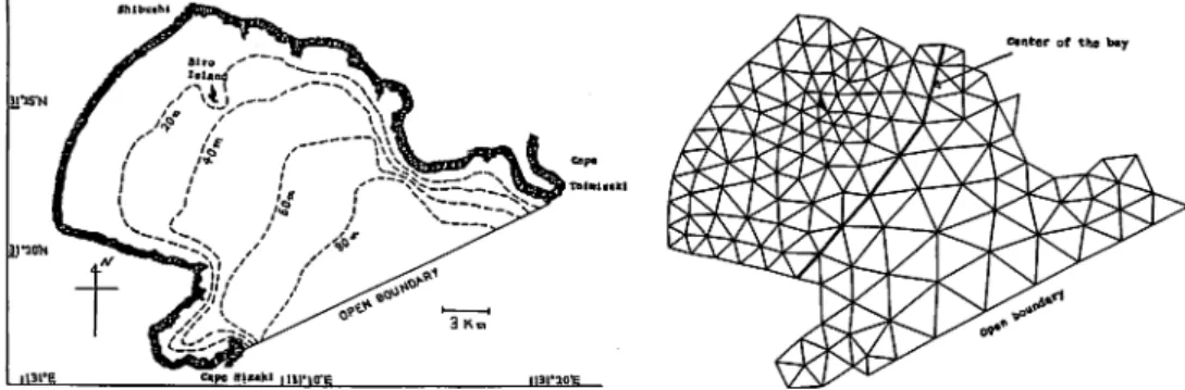
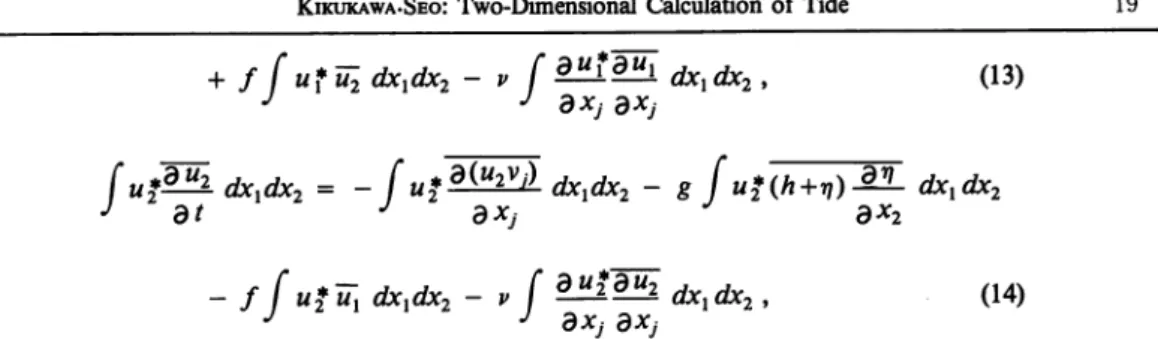
The geometry of Shibushi Bay is given in Fig. 1. Shibushi Bay has an almost square shape and, in the inner part of the bay there is Biro Island. It is opened to the Pacific Ocean in the east and the length of open boundary is about 20 km. The division of Shibushi Bay into the two-dimensional simplex elements is shown in Fig. 2. The number of the elements is 241 and the number of nodes is 148. The real depths at every node are read out from the chart.

Fig. 1. The geometry of Shibushi Bay.

ctnter of tha b»y

Fig. 2. The division of Shibushi Bay into the two-dimensional simplex elements.

16 Mem. Fac. Fish., Kagoshima Univ. Vol. 33, No.l (1984)

Some discussions about the stability of the calculational scheme are inevitable. Gray and

Lynch8* investigated the stability conditions for the one-dimensional tidal flow equations without

nonlinear advective terms. They found that the time difference At is limited by

At < At<

1 (AXminf

1 AXmin

VT Vgh

(ID (12)

in the case of Galerkin's finite element method with the two-step Lax-Wendroff time differentia tion scheme. As can be seen from Fig. 2, the minimum value of Ax is given around Biro Island to be Axmin = 700m. The value of the kinetic eddy viscousity coefficient v adopted in this article

is 102 (m2/s). Then Eq. (12) gives the more severe restriction for the time difference than Eq. (11). If the depth around Biro Island is taken to be 40m, the upper bound for the time difference estimated from Eq. (12) is about 20.4 seconds. Actually, however, the unstable divergence occurs if Af is chosen to be 20 seconds. The more regorous restriction than Eq. (12) might be caused by the two-dimensionality of our problem and/or the inclusion of the nonlinear advective terms. Calculation is performed by taking 15 seconds for the time difference, which gives the stable results.

The non-slip boundary condition is adopted at the coast in the hope to evaluate the tidal residual flow caused by the viscous boundary layer, although our division is still rough. At the entrance of Shibushi Bay, the water surface elevation is given as the harmonic oscillation with the amplitude lm and the period 12.5 hours. All other effects, e.g. the ocean current, the wind stress, the river current, the bottom stress, etc. are all out of our consideration.

(i) Owing to the oscillatory boundary condition at the open boundary, the water mass transport integrated over one tidal period (WMT) at any cross section of the bay must be vanished. In other words, the inflow part of WMT (WMTIN) and that of the outflow part (WMTOUT) have to be equal to each other. Calculation is performed over nine periods. The time variations of WMTIN and WMTOUT at the open boundary and at the center of the bay shown in Fig. 2 are represented

'(rrr/sec)

)r60-*

OPEN BOUNDARY

CENTER OF THE BAY

7 8 9

PERIOD

Fig. 3. WMTIN ( • ) and WMTOUT ( x ) at the open boundary (dashed line) and at the center of the bay (solid line), with respect to period calculated by EWM.

in Fig. 3. WMTIN and WMTOUT are almost equal after the 7-th period. It can be seen from Fig. 3 that WMTIN (or WMTOUT) at the center of the bay is about ten times less than that at the open boundary.

(ii) The distribution of the tidal residual water mass transport at the ninth period is represented in Fig. 4. There exists a small clockwise vortex around Biro Island and a large anti-clockwise one

at the south of Biro Island.

(iii) The distribution of the tidal residual velocity at the ninth period is represented in Fig. 5. There

exists a large anti-clockwise vortex at the south of Biro Island similar to Fig. 4. However, the

clockwise vortex does not appear around Biro Island, which is the main difference of Fig. 5 from Fig. 4.

(iv) In Fig. 6 is given the tidal residual water mass transport - tidal residual velocity x depth, the main part of which is the Stokes transport. There are characteristic north-east vectors at the

north of Biro Island.

(v) In Fig. 7 is given the averaged water surface elevation. Around Biro Island and at the south

of Biro Island, there appear the low water surface regions.

0.5 x10 (m'/sec)

Fig. 4. The distribution of the tidal residual water mass transport at the ninth period calculated by EWM.

0.5x10"tm'/sec) Fig. 6. The distribution of the tidal residual

water mass transport - tidal residual velocity x depth at the ninth period calculated by EWM.

0.5 xlOH(cm^sec) Fig. 5. The distribution of the tidal residual

velocity at the ninth period calculated by EWM.

Fig. 7. The distribution of the time averaged

water surface elevation at the ninth

period calculated by EWM. The shad ed (unshaded) area denotes the high (low) water surface region.

(vi) The distribution of the tidal velocity at t=6.25 hour and at t = 12.5 hour are represented in

18 Mem. Fac. Fish., Kagoshima Univ. Vol. 33, No.l (1984)

(vii) The hodographs at several points in the bay are represented in Fig. 9. Except the points of 5 and 7, they rotate clockwise. The velocity vectors with respect to time are shown in Fig. 10,

where the ordinate denotes the north-south direction.

t-6.25(houn

4(cnvsec) x / ^ x \ \ 4(cmxsec)

Fig. 8. The velocity distributions at t=6.25 hour and at f=12.5 hour calculated by EWM.

4(cmxsec)

Fig. 9. The hodographs at several points in the bay calculated by EWM. t=12.5(houO _g£_c

^m\F" *"

- v ^WTn ^ ^ " n , ^^^. «k&K\\\\\\\\>i.,..

V°°ir^

4H"20 N0=8 s e ^^$$m^\\\\v,. •50 scf-W ^ c«sS8MS\\\\w _{rtSS§^S^^v>^} N0=9 ' «££" 0Z> 60" 6JT

Fig. 10. The velocity vectors with respect to time for the points denoted in Fig. 9,

calculated by EWM.

(viu) Multiplying to Eqs. (1) and (2) by the weighting functions w*i and u*2 with the form of Eq. (4) respectively and averaging by the time, it follows

f Uf^^-dxldx2 = -fuf3^1^ dx1dx2 - g [uUh+ti)-^ dxxdx>

+/ f'ux*u2dxxdx2 - v f ^±^ildx1dx2t

0

J

J dXj dXj

fuf^2 dxxdx2 = - fuS^Wjl dxxdx2 - g fU2*(h+r,)£i- dxxdx:

J

dt

J

dXj

J

ax2

f f u$ux dxxdx2 - v f ^l^ldxxdx2i

J

J dXj dXj

(14)

where bar denotes the time averaging. The left hand sides of Eqs. (13) and (14) should be vanish

ed when the calculation is attained to give cyclic solutions. The four terms in the right hand sides

of Eqs. (13) and (14) willbe named asthe advective, the gravitational, the Coriolis and the viscous

termsrespectively. The distribution of each term is given in Fig. 11. The advective term is directed

to the inner part of the bay and has large values in the outer part of the bay. The gravitational

term is directed to the open boundary and has large values also in the outer part of the bay. The

Coriolis term is directed to the open boundary in the outer part of the bay and has a convergence

around Biro Island and a divergence at the south of Biro Island. The viscous term has small ab solute values all over the-bay. In Fig. 12 is given the normalized distribution of each term. The viscous term can be seen to be relatively large around Biro Island. In the inner part of the bay,

the advective term is valanced with the gravitational term and in the outer part of the bay, the

advective term, the gravitational term and the Coriolis term are balanced among them. Around Biro Island the advective, the gravitational and the viscous terms are balanced.

Advoctiveterm

i.OMO-Mcm'/set')

Gravitationalterm

l.oxio'(«n'/sec)

Viscoustarn

Fig. 11. The distributions of the advective, the gravitational, the Coriolis and the viscous terms

20 Mem. Fac. Fish., Kagoshima Univ. Vol. 33, No.l (1984)

Fig. 12. The distribution of the advective, the gravitational, the Coriolis and the viscous terms nor malized by themselves.

§4. Discussion

The two-dimensional tidal equations are solved by EWM for Shibushi Bay. The tidal residual flow and the balances of the terms in the time averaged Euler's equations of momentum are estimated. The division of the bay by the two-dimensional simplex elements is very much elude as shown in Fig. 2. We afraid that the viscous term would become more important when the finer division of the bay is adopted.

This article is only a preliminary work, because the ocean current, the wind stress, the river current, the bottom stress etc. are all out of our consideration. The effects must be important and have to be accounted in the future work. It is reported in Ref. 9) that the maximum water velocity at 5m depth is about four or five times larger than that estimated in this article and that the distribution of the time-independentvelocity at 5m depth is much more complex than Fig. 5

with about one hundred times larger absolute value.

References

1) G.Grotkop (1973): Finite element analysis of long-period water waves. ComuterMeth. Applied Mech.

Enging., 2, 147-157.

2) M.Kawahara and K.Haseoawa (1978): Periodic Galerkin finite element method of tidal flow. Int. Jour. Numer. Meth. Enging., 12, 115-127.

3) O.C.ZiENKffiwicz (1977) "The Finite Element Method" third Eddition, pp.535-539, (McGraw-Hill, Lon don, England).

4)

M.Kawahara, H.Hirano, T.Tsubota and K.Inaoaki (1982) Selective lumping finite element method for

shallow water flow, Int. Jour. Numer. Meth. Fluid. 2, 89-112.

5)

H.KncuKAWA and H.Ichikawa (1984): Animproved explicit finite element method for tidal flow. Int. Jour.

Numer. Meth. Enging. 20, 1461-1475.

6)

H.Kdcukawa (1983): Numerical calculation of tide in Kagoshima Bay part 2. Two-dimensional explicit

weighted residual method. Mem. Fac. Fish. Kagoshima Univ., 32, 29-48.

7)

M.A.E.Eisenbero and L.E.Malvern (1973): On the finite element integration in natural coordinates.

Int. Jour. Numer. Meth. Enging, 7, 574-575.

8)

W.G.Gray and D.R.Lynch (1977): Time-stepping schemes for finite element tidal model computations.

Adv. Water Resour., 1, 83-95.