A Simple Neural Network Model for Temporal Pulse Coding (Invariants of Dynamical Systems and Applications)

(1)

A Simple Neural Network

Model for

Temporal

Pulse

Coding

東大工学部計数数理–研

&CREST

渡辺正峰 (Masataka Watanabe)

東大工学部計数数理–興

&CREST

合原–幸 (Kazuyuki Aihara)

1 Introduction

In recent years there has been renewal of interest in the basic coding principle of the brain, how information is transmitted among neurons. Today, there are two major hypothesis: rate coding, where the mean firing rate is the carrier of information, and temporal coding, where timing of individual pulses are the carriers of information.

Rate coding hypothesis has been the established theory for a long time and most

model approaches aswell as many experiments on biological networks have been based

on this idea. This hypothesis was widely accepted due to the existence ofa

quantita-tive relationship between the firing rates of single cortical neurons and psychophysical judgments made by behaving monkeys(Barlow 1987; Newsome 1989; Britten 1992).

On the other hand, spatio-temporal coding has been recently brought to light by both biologists and theorists. Softky and Koch (1993) reported that the inter-spike

in-tervals of cortical pyramidal cells are highly variable and concluded that

neurons

func-tion

as

coincidence detectors which indicates temporal coding. Furthermore, Vaadia

et.$al$ observed the dynamical modulation of temporal relations between the discharges

of neurons in the monkey prefrontal cortex in response to contexts or external events,

leading to the idea that information is contained in the spike timing(Vaadia 1995). On

the theoretical side, Abeles proposed the notion of “synfire chains” which as

sures

the

timing accuracyof neuronal firings observed in brains of behaving monkeys with rather

unreliable

neurons

$(\mathrm{A}\mathrm{b}\mathrm{e}\mathrm{l}\mathrm{e}\mathrm{s}1993\mathrm{b})$. Besides this, many other experimental results and

theoretical considerations support temporal pulse coding in the brain($\mathrm{s}_{\mathrm{a}\mathrm{k}}\mathrm{u}\mathrm{r}\mathrm{a}\mathrm{i}$ 1993;

(2)

We believe that the truth lies somewhere in the between of pure rate coding and

pure temporal coding. However, we feel that it is also necessary to simplify things in

order to carry out theoretical studies, such as viewingthe coding ofthe brain fromthe two extremes, the rate coding and temporal coding hypothesis. The problem is that there seems to be onIy few fundamental models whichgive a mathematicaldescription of the underlying dynamics in temporal pulse coding. Whereas in the rate coding paradigm, say, we have the Hopfield model(Hopfield 1982). Hopfield introduced the notion of “energy” in a single layer neural network and showed that the neuronal dynamics evolves

so

that

energy

decreases with time.

The purpose of this paper is to introduce a simple model which describes

mathe-matically the ongoing dynamics of temporal pulse coding. That is to say, we will try to purely extract the effects of incident pulse timing on network dynamics and also make it simple enough for theoretical analysis. To be more specific, we eliminate the effects of spatial summation of neuronal activities, which was the key to rate coding, by using “uniform” synaptic strength on amutually connected network. Also we make

several assumptions

so

that we

are

able to define “network state”in such continuous time systems and thus describe the dynamics by iteration of maps.

We will first give the descriptions of the proposed model and next analyze the model by

means

of numerical simulation from the aspects of dynamical stability and basins of attraction. Furthermore, we introduce a learning rule which increases the stability and basin ofattraction of attractors in our proposed model. Final section is assigned

to discussions.

2 Neural Network Model

The network model is a deterministic point process model $\mathrm{b}\mathrm{a}s$ed on temporal pulse

coding. That is to say, pulses actually propagate among neurons with finite delay, and

neurons

work

as

coincidence detectors of incident pulses. Furthermore, in order

(3)

to extract the effect ofincident pulse timings

on

neuronal interaction, we

assume

that

neurons are

mutually connected with “uniform” synaptic efficacy. This corresponds to

the

case

where only

one

pattern is embedded in the network by the Hebbian learning

rule, whichis not very interestingfrom theview point of classical ratecoding. However, in atemporal pulse coding network model, by assuming random time delay for pulse propagation, it has been reported to show various dynamics($\mathrm{w}\mathrm{a}\mathrm{t}\mathrm{a}\mathrm{n}\mathrm{a}\mathrm{b}\mathrm{e}$ and Aihara

(1997), Watanabe et. $al$ (1998)$)$

.

Before giving equations and going into the details of the model, we take up the two assumptions which

we

make to construct

a

“simple

as

possible” model. The first

is that neuronal firings

are

localized in time. We realize this by setting the variance

of pulse propagation delay small enough so that pulses sent from a

group

of firing

neurons

_{do not spread out in time and overlap with pulses sent out from other} _groups

of neuronal firings. We call this group of pulses, “pulse group” As a consequence,

localized neuronal firings become

a

function ofthe previous localized neuronal firings,

that is to say, it becomes possible to describe the network dynamics in discrete steps

of pulse

groups.

The second assumption is to fix the number of firing

neurons

resultingfrom asingle pulse

group.

We

assume

some

kind of

a

negative feedbackloopwhichkeeps

a

moderate

rate of activity in the network. As a consequence, the network state becomes a fixed

dimensional vector and the dynamics

can

be written as iterations ofmaps.

Now that

we are

ready,

we

will

go

onto the details ofthe model, first in the general

case.

We define $\mathrm{t}^{f}(k)$

as

the neuronal firing time vector with firing time of _$N$

neurons

in the $k\mathrm{t}\mathrm{h}$ pulse

group

as its components.

As we stated earlier, only $n_{f}$

neurons

fire

in a single pulse group, so $n_{f}$ components have actual firing time as its value and rest

will be “_{$- 1$}” _indicating

that the

neuron

did not fire in the $k$ th pulse group. Fromthis

neuronalfiringvector, matrixof pulse arrivaltime in the $k+1\mathrm{t}\mathrm{h}$pulse group _{$\mathrm{T}^{P}(k+1)$}

(4)

$\mathrm{T}^{p}(k+1)=F(\mathrm{t}^{f}(k), \mathrm{D})$, (1)

where function $F$ adds pulse propagation delay given by the delay matrix$\mathrm{D}$ to the

neuronal firingtime

as

follows,

$t_{ij}^{p}(k+1)=\{$

$t_{j}^{f}(k)+d_{ij}$, $\mathrm{i}\mathrm{f}t_{j}^{f}\geq 0$,

$-1$, $\mathrm{i}\mathrm{f}t_{j}^{f}=-1$

.

(2) Here, $t_{ij}^{p}(k+1)$ and $d_{ij}$ are the components ofmatrix $\mathrm{T}^{p}(k+1)$ and $\mathrm{D}$, denoting

pulse arrival time and pulse propagation delay from pre-neuron $j$ to post-neuron $i$, respectively.

Given the pulse arrival time of all neurons in the network, the neuronal firingtime

of the $k+1\mathrm{t}\mathrm{h}$ pulse group is determined,

$\mathrm{t}^{f}(k+1)=G(\mathrm{T}^{p}(k+1))$. (3)

Here, the role of function $G$ is to determine “which neurons” and “when” to fire

given the distribution of pulses. Thus the selection of this function decides the property

of a single neuron and the negative feedback loop for stabilizing activity. Taking

equations (1) and (3) into account, the overall dynamics of

our

model

can

be written as

$\mathrm{t}^{f}(k+1)=G\mathrm{o}F(\mathrm{t}^{f}(k), \mathrm{D})$. (4)

describe the definite case used in the following simulations where,

as

the

most simple case, we choose the number of firing neurons in a pulse group $n_{f}=2$ and

function $G$ as described below.

The first part offunction $G$ is to decide which

neurons

to fire. Defining $\phi(1, k)$ and

(5)

choose the next two firing

neurons

with the smallest two incident pulse interval$(IPI)$

as,

$IPI_{i}(k+1)=|t_{\phi(1,k),i}^{p}(k+1)-t_{\phi}^{p}((2,k),ik+1)|=|\triangle t^{f}(k)+d_{\phi(1,k}),i-d_{\phi(2,k}),i|$, (5)

$IPI_{\emptyset(1}1,k+)(k+1),$$IPI_{\emptyset}(2,k+1)(k+1)<IPI_{i}(k+1)(i=1, \ldots, N, i\neq\phi(1, k+1), \phi(2, k+1))$,

(6) where $\triangle t^{f}(k)=t_{\phi(1,k}^{f}()k)-t_{\phi(k}^{f}(2,)k)$. This method of choosing neurons to fire

reflects the idea that

neurons

act ascoincidence detectors of incident pulses in temporal pulse coding.

Now that we know which neurons to fire in the $k+1$ th pulse group, the next role

of function $G$ is to determine “when” to fire. The firing time is a function of the local

information available to a neuron, the pulse arrival time, as follows,

$t_{i}^{f}(k+1)=(t_{\phi(1,k)}^{p},i+t_{\phi(2,k)}^{p},i)/2+a|t^{p}t_{\phi(2}^{p},|^{\gamma}\phi(1,k),i^{-}k),i(i=\phi(1, k+1),$$\phi(2, k+1)),$ $(7)$

where the first term of the right hand side takes the average of arrival time of the two pulses and the second term describes the firing delay depending on IPI. Larger the IPI, larger the firing delay. The two parameters $a$ and $\gamma$ characterizes the property of

the firing delay. These two values and the delay matrix are the only parameters in our

model and as we will see in the followingsection, especially $a$ has alarge influence

on

the network dynamics.

From equations(2) and (7), we get the following equation which corresponds to eq.

(4) in

the

general case,

(6)

$+a|t_{\phi(1}^{f},-k)t^{f}+k)d_{\phi}(1,k),i-d_{\phi}(2,k),i \int^{\gamma}\phi(2$

,

$(i=\phi(1, k+\dot{1}),$$\phi(2, k+1))$. (8)

Moreover, subtracting $t_{\phi(1)}^{f}1,k+(k+1)$ from $t_{\phi(1}^{f}2,k+$

)$(k+1)$, we get

$\triangle t^{f}(k+1)$ _$=$ _{$(d_{\phi(1,k)},\phi(1,k+1)+d\phi(2,k),\emptyset(1,k+1)-d_{\phi(}1,k),\phi(2,k+1)-d\phi(2,k),\emptyset(2,k+1))/2$}

$+a|\triangle t^{f}(k)+d_{\phi(}1,k),\phi(1,k+1)-d\phi(2,k),\phi(1,k+1)|^{\gamma}$

$-a|\triangle t^{f}(k)+d_{\phi}(1,k),\phi(2,k+1)-d_{\phi(2},k),\phi(2,k+1)|^{\gamma}$. (9)

Notice that from equations (6) and (9), the iteration of the map only depends

on

$\triangle t^{f}(k)$ and _{$\phi(1, k),\phi(2, k)$}. Therefore we can consider the network state of the _$k$ th

pulse group as the following three dimensional vector,

$\mathrm{s}(k)=\{\triangle t^{f}(k), \phi(1, k), \phi(2, k)\}$. (10)

Furthermore, without losing generality, we can map this three dimensional state

space onto one dimension which makes it possible to view the mapping,

$S(k)=\Delta t^{f}(k)+\psi\{\phi(1, k), \phi(2, k)\}$, (11)

where $\psi$ is a function such as,

$\psi(i,j)=2\Delta t_{\max}^{f}\{(2N-1)(i-1)/2+j-i\}$. ₍₁₂₎

Taking equations (9)(11) into account, the overall dynamics of

our

network with

$n_{f}=2$ becomes a

one

dimensional return map.

. _{$s(k+1)=\Omega(S(k), \mathrm{D})$}_, ₍₁₃₎

(7)

$+a|s(k)-\psi\{\phi(1, k), \phi(2, k)\}+d_{\emptyset}(1,k),H_{1}(S(k))-d\phi(2,k),H_{1}(s(k))|^{\gamma}$

$-a|S(k)-\psi\{\phi(1, k), \phi(2, k)\}+d_{\emptyset}(1,k),H_{2}(s(k))-d\phi(2,k),H_{2}(s(k))|^{\gamma}$

$+\psi\{H_{1}(S(k)), H_{2}(S(k))\}$. (14)

where $H_{i}(S(k))(i=1,2)$ is afunction which determines what

neurons

to fire from

the previous network state using equation (6).

3 Simulation

results

3.1 Change of

parameter

“

$\gamma$

”-piecewise linear and nonlinear

A network of$N=4$

neurons

with uniform random delay $(8<d_{ij}<12)$ is studied in

this section to investigate the change of dynamics with parameter “

$\gamma$

”

First,

we

will look at the return map of network states when $\gamma$ is 2. In this case,

$\mathrm{e}\mathrm{q}.(14)$ becomes,

$S(k+1)$ $=$ $2a(d_{\phi()}1,k,H_{1}(S(k))-d\phi(2,k),H_{1(S()}k))-d\phi(1,k),H_{1}(S(k))+d\phi(2,k),H1(S(k)))S(k)$

$+(d_{\phi(1,k)},H_{1}(s(k))+d_{\emptyset\{}2,k),H_{1}(s(k))-d\phi(1,k),H_{2}(S(k))-d_{\phi}(2,k),H2(s(k)))/2$

$+(d_{\phi(),(S}1,kH_{1}(k))-d\phi(2,k),H_{1}(S(k))))^{2}-(d\phi(1,k),H_{2}(s(k))-d\emptyset(2,k),H_{2(()}Sk)))^{2}$

$+\psi\{H_{1}(S(k)), H_{2}(S(k))\}=a\alpha(s(k), \mathrm{D})S(k)+\beta(S(k),\mathrm{D})$ , (15)

and since $H_{i}(S(k)$ stays constant for small changes of $S(k)$, it is a piecewise linear

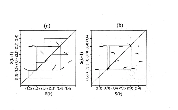
return map. Figure(1)$(\mathrm{a})$ shows the actual return map for $\gamma=2$.

On the other hand, Figure(1)$(\mathrm{b})$ shows the case for $\gamma=1.2$ where it becomes a

(8)

$\mathrm{O}(\mathrm{h}/$ $\circ \mathrm{t}^{\mathrm{x}}J$

Figure 1: Returnplot for (a) $\gamma=2.0$, piece-wise linear caseand (b) $\gamma=1.2$, piece-wise

nonlinear $\mathrm{c}\mathrm{a}\mathrm{S}\mathrm{e}(N=4, n_{f}=2,\overline{d}=10.0<d>=2.0)$

3.2 Change

of parameter

“$\mathrm{a}$”

-periodic,

chaotic

and complex

dynamics

In this subsection,

we

investigate the change of network dynamics with parameter $a$

which first appears in $\mathrm{e}\mathrm{q}.(7)$. As

we can

see from $\mathrm{e}\mathrm{q}.(14)$, parameter $a$ gives the

mean

inclination of the map. Therefore, increasing $a$ works to raise the

average

gradient of

the map, hence, the dynamics becomes less stable.

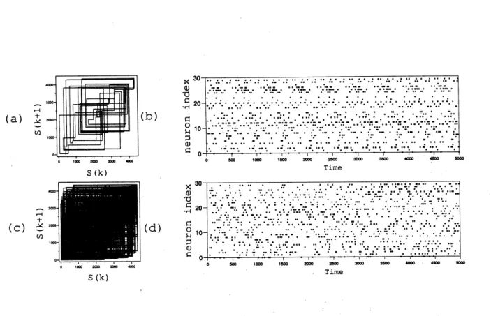
The neuronal firing of the network with two different $a$ is given in figure(2). As

we can see, the network dynamics is periodic for $a=0.5$ and chaotic for $a=5.0$.

Here we choosed 1.2 for $\gamma$ since the piecewise linear case $(\gamma=2.0)$ tends to break the

assumption which says that pulse

groups

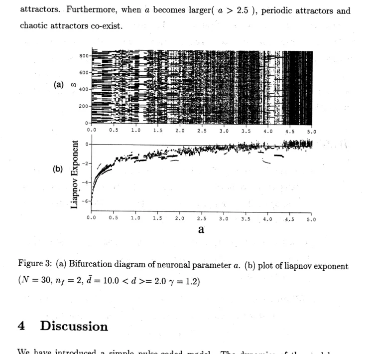
should not overlap when $a$ takes largevalues.

To get

a

whole grasp ofthe change of network behavior with $a$, we give

a

diagram

of bifurcation and lyapunov exponents in figure(3). Here, the lyapunov exponent is

(9)

(a)

3(K)

$\mathrm{S}(\mathrm{k})$

Figure 2: Return plot and Raster diagram $(\mathrm{a}),(\mathrm{b})$ periodic dynamics

:

$\mathrm{a}=0.05(\mathrm{c}),(\mathrm{d})$

chaotic dynamics: $\mathrm{a}=5.0(N=30, n_{f}=2,\overline{d}=10.0<d>=2.0\gamma=1.2)$

$\lambda=1/K\sum^{K-1}logk=0|dS(k+1)/dS(k)|$, (16)

$dS(k+1)/ds(k)$ $=$ $a\gamma\{|S(k)-\psi\{\phi(1, k), \phi(2, k)\}+d_{\phi(1,k),(S}H_{1}(k))-d\phi(2,k),H1(S(k))|^{\gamma-}1$

$-|S(k)-\psi\{\phi(1, k), \phi(2, k)\}+d_{\emptyset}(1,k),H_{2}(S(k))-d\phi(2,k),H_{2}(S(k))|\gamma-1\}$

$=a\gamma\{|t^{p}-\phi(2,k),\phi(1,k+1)t_{\phi()}p|1,k,\emptyset(1,k+1)-\gamma-1|t_{\phi(}^{p}-1,k),\phi(2,k+1)t_{\phi(}p|^{\gamma}2,k),\phi(2,k+1)-1$

$(1_{\mathfrak{l}}^{r}$

Calculation for

a

single $a$

was

started from

100

distinct initial states and plotted

after transient$(k> 10000)$_{. As parameter} $a$ increases, the lyapunov exponent

grad-ually rises and from the bifurcation diagram we

can see

that the network dynamics becomeschaotic. We should also notice the gap between multiple lyapunov exponents for single $a$ where they are negative. This indicates the existence of multiple stable

(10)

larger$(a>2.5)$ , periodic attractors and

chaotic attractors co-exist.

a

Figure

3:

(a)

Bifurcation

diagram ofneuronal parameter$a$. $(\mathrm{b})$ plot ofliapnovexponent

$(N=30, n_{f}=2,\overline{d}=10.0<d>=2.0_{\gamma}=1.2)$

4

Discussion

We have

introduced

a

simple pulse-coded _{model. The} _dynamics _{of the Model}

_was

clarified using a return map _{and the lyapunov exponent, where} _existence _of _periodic

and chaotic attractors

were

confirmed. It is alsoimportant to note that multiplestable

attractors exist in

our

model. We may consider these attractors as “memories”, as

in the Hopfield model. We have also proposed a learning rule which decreases the

lyapunov exponent of

an

_{attractor and hence}

_increases

_the _{stability and the} _basin _of

(11)

As we have stated earlier, this paper concentrated

on

the analysis of pure temporal

coding, in other words, we investigated only the effect of pulse timing

on

neuronal

interactions. Neuronal interactions, say, how

neurons

decide when to fire given the

outputs of other

neurons

in the network, is also

a

function of what

neurons

fired. This

is realized in the distribution of synaptic weights in usualmodels,whereas in

our

model

we

used an uniform distribution. Combining temporal and spatial effect

on

neuronal

interaction will be the subject of

our

future study.

References

[1] Abeles, M., Prut, Y., Bergman, H., Vaadia, E., Aertsen,A.M.H.J. (1993b) Integration, synchronicity and periodicity. In: Aertsen A. (ed) Brain

The-ory: Spatio-Temporal Aspects of Brain Function. Elsevier

Science

Publ.,

Amsterdam, New York, pp

149-181.

[2] Barlow, H.B., Kaushal, T.P., Hawken, M., Parker, A.J. (1987) Human

contrast discrimination and the threshold of cortical-neurons. J. Opt. Soc.

A, 4,

2366-2371.

[3] Britten K.H., Shadlen M.N., Newsome W.T., Movshon J.A. (1992) The

analysis of visual motion:

a

comparison of neuronal and psychophysical

performance. J. Neurosci, 12,

4745-4765.

[4] Hopfield, J.J. (1982) Neural networks and physical systems with emergent collective computational abilities. Proc. Natl. Sci. USA, 79, 2554-2558.

[5] Newsome, W.T., Britten, K.H., Movshon,

J.A.

(1989) Neural correlates

ofa perceptual decision. Nature, 341,

52-54.

[6] Sakurai, Y. (1996) Population coding by cell assemblies-what it really is in the brain. Neuroscience Research, 26,

1-16.

(12)

[7] Softky, W. R., Koch, C. (1993) The highly irregular firing of cortical cells

is inconsistent with temporal integration of random EPSPs. J. Neurosci,

13,

334-350.

[8] Vaadia, E., Haalman, I., Abeles, M., Bergman, H., Prut, Y., Slovin, H., Aertsen, A. (1995) Dynamics of neuronal interactions in monkey cortex in relation to behavioral events. Nature, 373, 515-518.

[9] Watanabe M., Aihara $\mathrm{K}.(1997)$ Chaos in neural networks composed of

coincidence detector neurons, Neural Networks, 10, 8,

1353-1359

[10] Watanabe M., Aihara K. and Kondo S. (1998) A dynamical neural net-work with temporal coding and functional connectivity,Biological Cyber-netics, 78,