Large-deviation approximations for the
discrete
distribution
筑波大数学
高橋邦彦
(Kunihiko Takahashi)
筑波大数学
$\text{赤平上文}$
(Masafumi Akahira)
1.
はじめに
統計的推測の高次漸近理論では
Edgeworth(
展開による
) 近似がよく用いられ,
推定量
,
検定などの高次の漸近的性質が論じられてきた
.
実際
, 推定量の真の母数の周りでの集中
確率を漸近的に求めるときには漸近分布の中心部分を必要とし,
そのとき
Edgeworth
近似
が重要な役割を果たした
$([\mathrm{B}\mathrm{C}89])$. –
方
,
Bahadur
効率は漸近分布の裾の部分に基づいて
いて
,
大偏差確率を必要とする.
また
,
裾確率の近似についてもいろいろ論じられている
(
$.[\mathrm{D}87]$,
[J95]).
.
本論では
,
独立な離散型確率変数の和の分布に対する大偏差
(
原理による
)
近似を高次の
次数まで求めて
, 通常用いられている正規近似
,
Edgeworth
近似と比較検討する
$([\mathrm{A}\mathrm{T}\mathrm{T}98])$.
2.
大偏差近似
$X_{1},$ $\cdots,$ $X_{n},$$\cdots$
を互いに独立に
,
各
$j=1,2,$
$\cdots$について
$X_{j}$が確率関数
$p_{j}(x)=P\{X_{j}=X\}$
$(_{X=0,\pm}1, \pm 2, \cdots)$
に従う離散型確率変数列とする.
それらの和
$S:= \sum^{n}j=1xj$
の確率関数を
$p_{n}^{*}(y)$
$:=P\{S_{n}=y\}$
$(y=0, \pm 1, \pm 2, \cdots)$
とする
.
また各
$j$について
,
$X_{j}$の積率母関数を
$M_{j}(\theta):=E[e^{\theta x_{j}}](\theta\in)-$
とする
.
ただ
し
$$
は原点を含むある開区間とする.
さて各月こついて,
確率関数
$p_{j_{)}\theta}(x):=P_{\theta}\{X_{j}=x\}=$
.
$.p_{j}(x)e.M\theta x.(\theta)^{-}1j$
$(x=0, \pm 1, \pm 2, \cdots)$
の離散指数型分布族
$P_{j},:=\{p_{j,\theta}..\cdot.(x) : \theta\in\}$を考える
.
ここで
$Pj,0(x)=pj(x)$
になる
.
また
$S_{n}$
の確率関数を
で表わす
.
ただし
$p_{n}^{*},\mathrm{o}(y)=p_{n}(*y)$とする
.
このとき
$p_{n,\theta}^{*}(y)=p^{*}n(y)e^{\theta}r.\backslash \cdot.yj=\prod_{1}M_{j(\theta})^{-}1$
(2.1)
となる. また各
$j$について,
乃の下で,
X,
の特性関数は
$E_{\theta}[e^{itX}j]= \sum_{x}e^{itx}pj,\theta(_{X})=Mj(\theta)^{-1}M_{j(\theta}+it)$
になる
. 従って
,
$\{P_{j}\}$の下で,
$S_{n}$の特性関数は
$E_{\theta}[e^{itS}]n= \prod_{j=1}M_{j(t)\prod_{j=}M_{j(}}\theta+i1\theta)^{-1}$
となるから,
フーリエ逆変換を用いて
$p_{n,\theta}*(y)= \frac{1}{2\pi}\int_{-}\prod_{\pi_{j=}1}^{\pi}M_{j(}n\theta+it)\prod_{j=1}^{n}$
$M_{j}(\theta)-1e$
-itydt
(2.2)
になる
.
そこで
(2.1),
(2.2)
から
$p_{n}^{*}(y)=e^{-} \prod_{j1}^{n}\theta yM_{j()\frac{1}{2\pi}}=\theta\cdot\int-\pi j=1=\prod_{j}\prod M_{j}(\theta+it)M_{j}(\theta)-1e$
$\pi nn1$
-itydt
を得る
.
ただし
$i$は虚数単位とする
.
また
$K_{n}( \theta):=\sum_{j1}^{n}=\mathrm{g}M_{j}\mathrm{l}\mathrm{o}(\theta)$とおくと
$p_{n}^{*}(y)=e^{K(\theta)\theta y}\mathfrak{n}-$
.
$\frac{1}{2\pi}\int_{-\pi}^{\pi}$$e^{K_{n}}(\theta+it\rangle$$-K_{n}(\theta)$
-itydt
(2.3)
になる
.
さらに
Taylor
展開によって
,
十分に小さい
$|t|$に対して
$K_{n}( \theta+it)-K_{n}(\theta)=K^{(}1)(n\theta)it+\frac{1}{2}K^{()}2(nit)2+\frac{1}{6}K(3)(n\theta)(it)3+\frac{1}{24}K^{()}4(n\theta)(it)^{4}+\cdots$
(2.4)
になる
. ただし各
$\alpha=1,2,$
$\cdots$について
$K_{n}^{(\alpha)}(\theta)=(d^{\alpha}/d\theta^{\alpha})K_{n}(\theta)$とする. このとき
,
$S_{n}=y(y=0, \pm 1, \pm 2, \cdots)$
に対して
$K_{n}^{(1)}(\hat{\theta})=y$となる
$\theta$の推定量
$\hat{\theta}:=\hat{\theta}(Sn)$
を考える
.
ここで
$K_{n}^{(\alpha)}(\hat{\theta})=o(n)(\alpha=2,3, \cdots)$
を仮定する
.
定理
1.
$S_{n}$の確率関数
$p_{n}^{*}(y)$は漸近的に次のように与えられる.
証明については,
$\int_{-\pi}^{\pi}$ $e^{K_{n}(})\hat{\theta}+it-K_{n}(\hat{\theta})$-itydt
..
$= \frac{1}{\sqrt{K_{n}^{(2)}(\hat{\theta})}}\int_{\sqrt{K_{n}^{(2)}(\theta)}}^{\pi^{\sqrt{K_{n}^{(2)}(\theta)}}}-\pi\exp\{K_{n}(\hat{\theta}+\frac{iz}{\sqrt{K_{n}^{(2)}(\hat{\theta})}})-K_{n}(\hat{\theta})-\frac{iyz}{\sqrt{K_{n}^{(2)}(\hat{\theta})}}\}dz$となるから,
(2.4)
と
$\hat{\theta}$の定義を用いて計算すれば結論を得る
.
..
各
$j=1,2,$
$\cdots$について, 確率関数
$Pj,\theta(\cdot)$と
$p_{j}(\cdot)$の間の
Kullback-Leibler
情報量を
$I_{j}( \theta, 0):=\sum_{x}pj,\theta(X)\log\frac{p_{j,\theta}(x)}{p_{j}(_{X)}}$
で定義する
.
このとき確率関数
$p_{j,\theta}^{*}(\cdot)$と
$p_{j}^{*}(\cdot)$の間の
Kullback-Leibler
情報量は
$I_{n}^{*}( \theta, 0)=\sum_{j=1}I_{j(}\theta,$
$0)=\theta K_{n}^{(1)}(\theta)-K_{n}(\theta)$
となる.
従って定理
1
から次の系を得る
.
系
.
$S_{n}$の確率関数
$p_{n}^{*}(y)$は漸近的に次のように与えられる.
$p_{n}^{*}(y)= \frac{1}{\sqrt{2\pi K_{n}^{(2)}(\hat{\theta})}}e-I_{n}^{*}(\dot{\theta},0)[1+\frac{K_{n}^{(4)}(\hat{\theta})}{8\{K_{n}^{(2)}(\hat{\theta})\}2}-\frac{5\{K_{n}^{(3)}(\hat{\theta})\}2}{24\{K_{n}^{()}(\hat{\theta})2\}3}+o(\frac{1}{n^{2}})]$
.
定理
2.
$S_{n}$の裾確率は漸近的に次のように与えられる
.
$P \{S_{n}\geq y\}=\frac{1}{\sqrt{2\pi K_{n}^{(2)}(\hat{\theta})}}e^{K_{n}(\overline{\theta})\hat{\theta}}-y\sum_{=z0}e\infty-\hat{\theta}z$
$+ \frac{K_{n}^{(4)}(\hat{\theta})}{8\{K_{n}^{(2)}(\hat{\theta})\}2}-\frac{5\{K_{n}^{(3)}(\hat{\theta})\}^{2}}{24\{K_{n}^{()}(\hat{\theta})\}23}+O(\frac{1}{n^{2}})]$
,
$y>E(S_{n})$
.
証明については
,
(2.3)
から任意の
$z\geq 0$
に対して
$p_{n}^{*}(y+\mathcal{Z})=eK_{n}(\hat{\theta})-\hat{\theta}(y+z)$
.
$\frac{1}{2\pi}\int_{-\pi}^{\pi}e^{K_{n}}-it(y+z)d(\overline{\theta}+it)-K_{n}(\hat{\theta})t$定理
2
の結果は
$y-E(S_{n})=o(n)$
のとき意味を持つことに注意したい.
しかしこのこ
とは,
通常
,
鞍部点近似
(saddlepoint approximation)
として
$y-E(\cdot S_{n})=o(n)$
のときに
正規分布に基づいて得た結果
(例えば
Lugannani
and
Rice
[LR80],
Robinson
[R82])
とは
異なっている
.
3.
二項分布の場合
$X_{1},$
$\cdots,$$X_{n},$$\cdots$
を互いに独立に
,
各
$j–1,2,$
$\cdots$について
$X_{j}$が二項分布
$B(1,p_{j})$
に従
う確率変数とする
.
ただし
$0<p_{j}<1$
とし,
また.
$q_{j}=1-p_{j}(j=1,2, \cdots)$
とする
.
この
とき各
$y=0,1,$
$\cdots,$ $n$について
$i$ $K_{n}^{(1)}( \theta)=\sum^{n}\frac{p_{j}e^{\theta}}{p_{j}e^{\theta}+qj}=j=1y$となる
$\theta$を
$\hat{\theta}$とする
.
このとき
$\hat{\tau}:=e^{\hat{\theta}}$とお 1,
$\backslash$て
, 各
$j\iota_{arrow}^{-}$ついて
p^j
$:=p_{j^{\hat{\mathcal{T}}}}/(p_{j^{\hat{\mathcal{T}}}}+q_{j})$,
$\hat{q}_{j}:=1-\hat{p}_{j}$
とすれば
,
$K_{n}^{(2)}( \hat{\theta})=\sum_{j=1}^{n}\hat{P}j\hat{q}_{j},$ $K_{n}^{(3)}( \hat{\theta})=\sum_{j=1}^{n}\hat{p}j.\hat{q}_{j}(\hat{q.}j-\hat{p}_{j}),$ $K_{n}^{(4)}(\hat{\theta})=$ $\sum_{j=1}^{n}\hat{p}j\hat{q}_{j()}1-6\hat{p}_{j\hat{q}_{j}}$になる
.
従って定理 1 から大偏差近似
$p_{n}^{*}(y)= \frac{1}{\sqrt{2\pi\sum_{j-1}^{n}-\hat{p}_{j\hat{q}j}}}(_{j=1}\prod^{n}\frac{q_{j}}{\hat{q}_{j}})\hat{\tau}-y$.
.
$1+ \frac{K_{n}^{(4)}(\hat{\theta})}{8(\sum_{j=1}^{n}\hat{p}j\hat{q}j)^{2}}-\frac{5\{K_{n}^{(3})(\hat{\theta})\}^{2}}{24(\sum_{j=1}^{n}\hat{p}j\hat{q}j)^{3}}+o(\frac{1}{n^{2}})]$を得る.
ここで上式の右辺の第
1
項目までの近似を
1
次の大偏差近似として
$LD_{1}$
と表わし,
右辺すべての項による近似を
2
次の大偏差近似として
$LD_{2}$
で表わす.
方
,
$S_{n}$の
$*=$
ムラントは
$\mu_{n}:=E(S_{n})=\sum_{1j=}^{n}p_{j}$
,
$v_{n}:=V(sn)= \sum_{=j1}$
pjq
$n$j,
$\kappa_{3,n}:=\kappa_{3(S_{n})}=\sum p_{j}qj(q_{j}-j=1np_{j})$
,
$\kappa_{4,n}:=\kappa_{4}(sn)=\sum j=1np_{jq_{j}(p}1-6jq_{j})$
となるから,
&
の分布の
Edgeworth
展開は
$P \{S_{n}=t\}=P\{\frac{S_{n}-\mu_{n}}{\sqrt{v_{n}}}=\frac{t-\mu_{n}}{\sqrt{v_{n}}}\}$ $= \frac{1}{\sqrt{v_{n}}}\phi(y)\{1+\frac{\kappa_{3,n}}{6v_{n}^{3/2}}(y-33y)+\frac{\kappa_{4,n}}{24v_{n}^{2}}(y-643y^{2}+)$$+ \frac{\kappa_{3,n}^{2}}{72v_{n}^{3}}(y^{6}-15y^{4}+45y-152)\}+o(\frac{1}{n\sqrt{n}})$
になる.
ただし
$y:=(t-\mu_{n})/\sqrt{v_{n}},$
$\phi(y)=(1/\sqrt{2\pi})e^{-y^{2}/}2$
とする
. 上式の右辺の第
1 項目までの近似を正規近似といい,
右辺のすべての項による近似を
Edgeworth
近似と
いう
.
このとき大偏差近似
$LD_{1},$
$LD_{2}$
はそれぞれ正規近似,
Edgeworth
近似より端にお
いて精確であることが分かる
. 実際
,
次の場合について数値計算を行って比較した
. (i)
$\{p_{j}\}_{j=1}^{9}=0.1$
(0.1)0.9,
(ii)
$\{p_{j}\}_{j^{9}1}^{1}==$0.05(0.05)0.95, (iii)
$\{p_{j}\}_{j=}^{10_{1}}=$0.05(0.05)0.50, (iv)
$\{p_{j}\}_{j=1}^{20}=0.03(\mathrm{o}.03)\mathrm{o}.60,$
$(\mathrm{v})\{p_{j}\}_{j=1}^{n}$が区間
$(0,1)$
上の一様乱数
$(n=10,20).,$
$(\mathrm{v}\mathrm{i})\{p_{j}\}_{j=1}^{n}$が区間
$(0.05, \mathrm{o}.95)$
上の
–
様乱数 $(n=10,20)$
(表
$3.1\sim 3.8$
参照).
また定理
2
より
$S_{n}$の裾確率は
$y>E(S_{n})$
に対して
$P\{s_{n}\geq y\}$
$=$
$\frac{1}{\sqrt{2\pi\sum_{j1}^{n}--\hat{p}_{j\hat{q}j}}}(\prod_{j=1}^{n}\frac{q_{j}}{\hat{q}_{j}})\hat{\mathcal{T}}-y$.
$[ \frac{1-\hat{\mathcal{T}}^{-(1)}m+}{1-\hat{\tau}^{-1}}\{1$$+$
$\frac{K_{n}^{(4)}(\hat{\theta})}{8(\sum_{j=1}^{n}\hat{p}_{j\hat{q}_{j})^{2}}}-\frac{5\{K_{n}^{(3)}(\hat{\theta})\}2}{24(\sum_{j1}^{n}=\hat{p}_{j\hat{q}_{j})^{3}}}.\}$ $- \frac{1}{2\sum_{j=1}^{n}\hat{p}_{j\hat{q}j}}\{-\frac{(m+1)^{2_{\hat{\mathcal{T}}}}-(m+1)}{1-\hat{\tau}^{-1}}$$+ \frac{1}{(1-\hat{\mathcal{T}}^{-}1)^{3}}(-(2m+3)\hat{\mathcal{T}}-(m+2)2m+1)\hat{\mathcal{T}}^{-(})+(m+3+\hat{\tau}-1(1+\hat{\tau}^{-1}))\}$
$- \frac{K_{n}^{(3)}(\hat{\theta})}{2(\sum_{j=1}^{n}\hat{p}_{j\hat{q}_{j})^{2}}}\{-\frac{(m+1)_{\hat{\mathcal{T}}}-(m+1)}{1-\hat{\tau}^{-1}}+\frac{(1-\hat{\tau}^{-})(m+1)\hat{\mathcal{T}}^{-1}}{(1-\hat{\mathcal{T}}^{-}1)^{2}}\}^{\backslash }+\backslash o(\frac{1}{n^{2}})]$
となる
.
ただし
$m=n-y$
とし
,
$K_{n}^{(3)}.( \hat{\theta})=\sum_{j=!}.\hat{p}_{j}\hat{q}.j(\hat{q}_{j}-n)\hat{p}_{j}$
,
$K_{n}^{(4)}( \hat{\theta})=\sum^{n}\hat{p}_{j}j=1\hat{q}_{j(}1-6\hat{p}j\hat{q}_{j})$方,
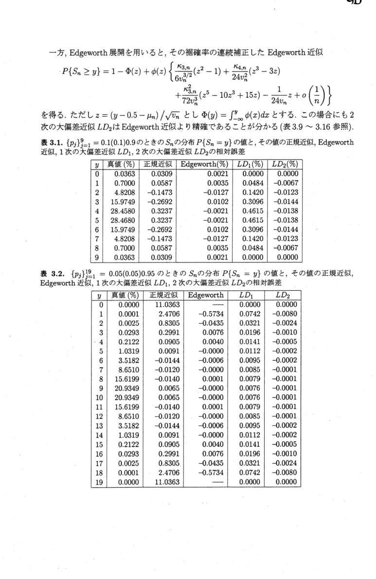
Edgeworth
展開を用いると, その裾確率の連続補正した
Edgeworth
近似
$P \mathrm{f}^{s_{n}\geq y}\}=1-\Phi(z)+\emptyset(Z)\{\frac{\kappa_{3,n}}{6v_{n}^{3/2}}(z^{2}-1)+\frac{\kappa_{4,n}}{24v_{n}^{2}}(_{Z}3-3Z)$
$+ \frac{\kappa_{3,n}^{2}}{72v_{n}^{3}}(z^{5}-1\mathrm{o}z+135z)-\frac{1}{24v_{n}}Z+O(\frac{1}{n})\}$
を得る
.
ただし
$z=(y-0.5-\mu n)/\sqrt{v_{n}}$
とし
$\Phi(y)=\int_{-\infty}^{y}\phi(X)dX$
とする
.
この場合にも
2
次の大偏差近似
$LD_{2}$
は
Edgeworth
近似より精確であることが分かる
(表 39\sim 3.16 参照).
表 3.1.
$\{p_{j}\}^{9}j=1=0.1(0.1)\mathrm{o}.9$
のときの
$S_{n}$の分布
$P\{s_{n}=y\}$
の値と
, その値の正規近似,
Edgeworth
表
33.
$\{pj\}_{j^{0}1}^{1}==$0.05(0.05)0.50 のときの
&
の分布
$P\{S_{n}=y\}$
の値と
, その値の正規近似,
Edgeworth 近似
,
1 次の大偏差近似
$LD_{1},2$
次の大偏差近似
$LD_{2}$
の相対誤差
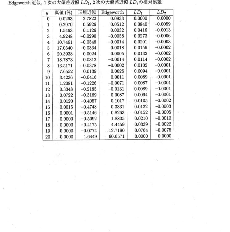
表 34.
$\{p_{j}\}_{j}^{20}=1=$0.03(0.03)0.60
のときの
$S_{n}$の分布
$P\{S_{n}=y\}$
の値と
,
その値の正規近似
,
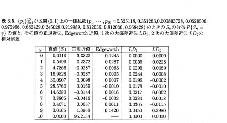
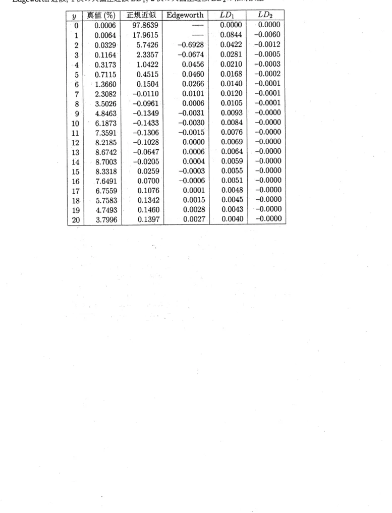
表 35.
$\{p_{j}\}_{j^{0}1}^{1}=$が区間
$(0,1)$
上の–様乱数
(
$p_{1},$$\cdots,p_{10=0.52}5118$
,
0.351263,0000803728, 0.0528506,
0.972966, 0.682429,0245028,0219989, 0.812036, 0.812036,
0.569428)
のときの
$S_{n}$の分布
$P\{S_{n}=$
$y\}$の値と
, その値の正規近
\’iJJ, Edgeworth
近似
,
1 次の大偏差近似
$LD_{1},2$
次の大偏差近似
$LD_{2}$
の
相対誤差
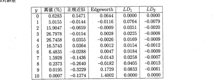
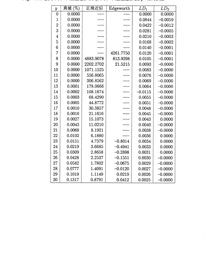
表
36.
$\{p_{j}\}_{j}^{20_{1}}=$が区間
{
$0,1)$
上の
–
様乱数
(
$p_{1},$$\cdots,p_{10}=0.305146$
,
0.715095,
0.612101,
0.672283,
0.447648,
0.268358,
0.434328, 0.552620, 0.608603, 0.130255, 0.941095, 0.141198, 0.164085,0693920,0565611,
0.
$977985,\mathrm{o}.0513902,0$$.877854,\mathrm{o}.451323$
,0.0628465)
のときの
$S_{n}$の分布
$P\{S_{n}=y\}$
の値と
,
その値
表
37.
$\{p_{j}\}_{j^{0}1}^{1}=$が区間
$(0.05, \mathrm{o}.95)$
上の–様乱数
(
$p_{1},$$\cdots,p_{1}0=$
0.120824, 0.58353, 0.441495,
0.17778, 0.447765, 0.185215, 0.197315, 0.484553, 0.206519,
0.747038)
のときの
$S_{n}$の分布
$P\{S_{n}=$
$y\}$の値と, その値の正規近似,
Edgeworth
近似, 1
次の大偏差近似
$LD_{1},2$
次の大偏差近似
$LD_{2}$
の
相対誤差
表 38.
$\{p_{j}\}_{j1}^{20}=$が区間
$(0.05, \mathrm{o}.95)$
上の–様乱数
(
$p_{1},$ $\cdots’,$$P10=$
0.865169, 0.760194, 0.163742,
0.862702, 0.903511, 0.504386, 0.706864, 0.921407, 0.150022, 0.139438, 0.587975, 0.469021, 0.941708,
0.191839, 0.168768, 0.500518, 0.138714, 0.217245,
0.060993,
0.462495)
のときの
$S_{n}$の分布
$P\{S_{n}=$
$y\}$の値と, その値の正規近似,
Edgeworth
近似, 1 次の大偏差近似
$LD_{1},2$
次の大偏差近似
$LD_{2}$
の
相対誤差
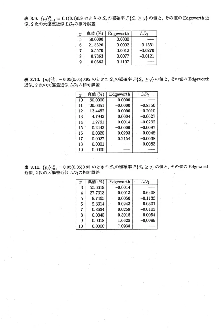
表 39.
$\{p_{j}\}_{j=1}^{9}=0.1$
(0.1)0.9
のときの
$S_{n}$の裾確率
$P\{S_{n}\geq y\}$
の値と,
その値の
Edgeworth
近
似
,
2
次の大偏差近似
$LD_{2}$
の相対誤差
表 310.
$\{p_{j}\}_{j=1}^{1\mathfrak{g}}=0.05(\mathrm{o}.05)0.95$のときの
$S_{n}$の裾確率
$P\{S_{n}\geq y\}$
の値と
,
その値の
Edgeworth
近似
,
2
次の大偏差近似
$LD_{2}$
の相対誤差
表 311.
$\{p_{j}\}_{j^{0}1}^{1}==0.05(\mathrm{o}.05)\mathrm{o}.95$のときの
$S_{n}$の裾確率
$P\{S_{n}\geq y\}$
の値と
,
その値の
Edgeworth
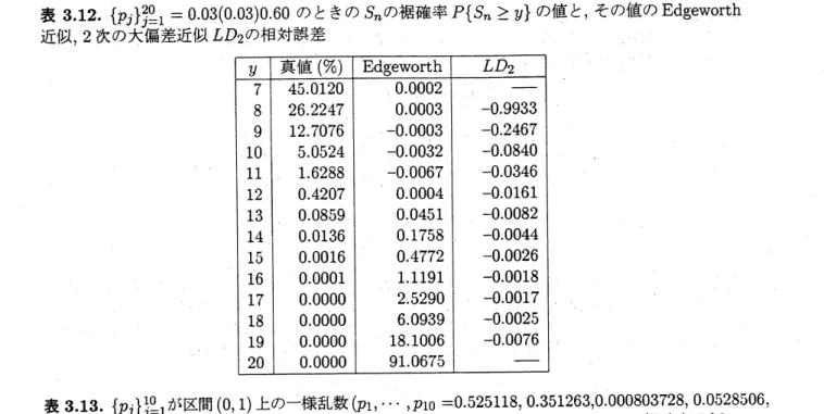
表
312.
$\{p_{j}\}_{j=1}200.0=3(\mathrm{o}.03)\mathrm{o}.60$のときの
$S_{n}$の裾確率
$P\{S_{n}\geq y\}$
の値と
,
その値の
Edgeworth
表 315.
$\{p_{j}\}_{j=}101$が区間
$(0.05, \mathrm{o}.95)$
上の
–
様乱数
(
$p_{1},$$\cdots,P10=$
0.120824,
0.58353, 0.441495,
0.17778, 0.447765,
0.185215.
0.197315,
0.484553,
0.206519,
0.747038)
のときの
$S_{n}$の裾確率
$P\{S_{n}\geq$
$y\}$の値と,
その値の
Edgeworth
近似
, 2
次の大偏差近似
$LD_{2}$
の相対誤差
表 316.
$\{Pj\}_{j^{0}1}^{2}=$が区間
$(0.05, \mathrm{o}.95)$
上の–様乱数
(
$p_{1},$$\cdots,P10=$
0.865169, 0.760194, 0.163742,
0.862702, 0.903511, 0.504386, 0.706864, 0.921407, 0.150022, 0.139438, 0.587975, 0.469021, 0.941708,
0.191839, 0.168768, 0.500518, 0.138714, 0.217245, 0.060993,
0.462495)
のときの
$S_{n}$の裾確率
$P\{S_{n}\geq y\}$
の値と,
その値の
Edgeworth
近似,
2 次の大偏差近似
$LD_{2}$
の相対誤差
4.
負の二項分布の場合
確率変数
$X_{1},$$\cdots,$$X_{n},$$\cdots$を互いに独立に
,
各
$j=1,2,$
$\cdots$について
,
$X_{j}$が
$f_{X_{j}}(x)=P\{X_{j}=x\}=p_{jj}^{r_{jx}}q$
を確率関数とする負の二項分布
$NB(r_{j,Pj})$
に従うとする
.
ただし
$0<p_{j}<1$
とし,
また
$q_{j}=1-p_{j}(j=1,2, \cdots)$
とする.
このとき
$S_{n}= \sum_{j=1j}^{n}X$
の分布とその大偏差近似
,
正規
近似
,
Edgeworth
近似をそれぞれ求めて数値的に比較する
.
$(\mathrm{i})S_{n}$の分布
:
$S_{n}$の分布は次のようにして再帰的に得られる
.
例えば
$n=20,$
$r_{j}=r$
$q_{16}=\cdots=q20=d$
の場合
,
$P \{X_{j}=x\}=\frac{r(r+1)\cdots(r+X-1)}{x!}a^{r}(1-a)^{x}$
$(x=0,1,2, \ldots ; j--1, \ldots, 5)$
,
$P \{x_{j}=X\}=\frac{r(r+1)\cdots(r+X-1)}{x!}br(1-b)x$
$(x=0,1,2, \ldots ; j=6, \ldots, 10)$
,
$P \{X_{j}=X\}=\frac{r(r+1)\cdots(r+x-1)}{x!}c(r1-C)^{x}$
$(x=0,1,2, \ldots ; j=11, \ldots, 15)$
,
$P \{X_{j}=x\}=\frac{r(r-+1)\cdots(r+X-1)}{x!}d^{r}(1-d)^{x}$
$(x=0,1,2, \ldots ; j=16, ’.
.
, 20)$
となる
.
ここで
Si
$:=S_{5}= \sum_{j}5x=1j,$
$S_{2}’:= \sum_{j=6}^{10}Xj,$
$S_{3}’:= \sum_{j1}^{15}=1x_{j},$
$S_{4}’:= \sum_{j=}20_{16}Xj$
と
おくと
$S_{1’ 2}^{\prime s^{\prime s’}},3$’
$S_{4}’$はそれぞれ負の二項分布
$NB(5r, a),$ $NB(5r, b),$ $NB(5r, c),$ $NB(5r, d)$
に従う.
S\’i
と
$S_{2}’$は互いに独立なので
$S_{1}’+S_{2}’$
の確率関数は次のようになる
.
$P\{S_{1}’+S_{2}’=0\}=P\{S_{1}’=0\}P\{S’2=0\}=a^{5r}b^{5r}$
,
$P\{S_{1}’’+s_{2}=1\}$
$=$
$P\{S_{1}’=1\}P\{s_{2}’=0\}+P.\{S_{1}’=0\}P\{S_{2}’=1\}$
$=$
$5ra^{5r_{b^{5r}(2}}-a-b)$
,
$P\{S_{1}’+S’2=2\}$
$=$
$P\{S_{1}’=2\}P\{S^{;}2=0.\}+P\{S_{1}’-arrow 1\}P\{S’2=1\}+P\{S_{1}’=0\}P\{S^{r}2=2\}$
$=$
$5ra^{5r}b^{5r} \mathrm{t}\frac{5r+1}{2}(1-a)2+5r(1-a)(1-b)+\frac{5r+1}{2}(1-b)^{2}\}$
$P\{s_{1^{+}}’s’2=3\}$
$=$
$P\{S_{1}’=3\}P\{S_{2}’=0\}+P\{S_{1}’=2\}P\{s_{2}’=1\}+P\{S_{1}’=1\}P\{s_{2}’=2\}$
$+P\{S_{1}’=0\}P\{s_{2}’=3\}$
$=$
$5r(5r+1)a^{5r}b^{5r} \{\frac{1}{6}(5r+2)(1-a)^{3}+\frac{5}{2}r(1-a)^{2}(1-b)$
$+ \frac{5}{2}r(1-a)(1-b)2+\frac{1}{6}(5r+2)(1-b)^{3\}}$
ここで
$S_{12}’:=S_{1}’+S_{2}’$
とおくと
$S’s’s1^{+}2^{+}31’=s’S’2^{+}3$
.
となり.
$S_{12}’$と
$S_{3}’$も互いに独立なので上と同様にして
$S_{12}’+S_{3}’=s_{1}’+S_{2}’+S_{3}’$
の確率関
数が得られる
.
さらに同様の手順を繰り返すことで
$S_{1}’+S_{2}’+S_{3}’+S_{4}’$
の確率関数を得る
.
(ii)
大偏差近似
:
各
$j=1,2,$
$\cdots$について,
$|\theta|$が小さいとき
X,
の積率母関数は
$M_{j}(\theta)=E(e^{\theta X_{j}})=p_{j}^{r_{j}}(1-q_{j}e)\theta-r_{j}$
で与えられる. このとき
$K_{n}( \theta)=\sum_{j=1}^{n}\log M_{j}(\theta)=\sum_{j=1}^{n}\{rj\log p_{j}-r_{j}\log(1-q_{j}e^{\theta})\}$
であるから,
各
$y=0,1,$
$\cdots$について
$K_{n}^{(1)}( \theta)=\sum_{j=1}^{n}\frac{r_{jq_{j}}e^{\theta}}{1-q_{j}e^{\theta}}=y$となる
$\theta \text{を}\hat{\theta}$とする
.
ここで
,
$\hat{\tau}=e^{\hat{\theta}}$とおくと
$y= \sum_{j=1}^{n}\frac{r_{j}q_{j^{\hat{\mathcal{T}}}}}{1-q_{j^{\hat{\mathcal{T}}}}}$になる
.
また
$K_{n}^{(2)}( \hat{\theta})=\sum^{n}\frac{r_{jq_{j^{\hat{\mathcal{T}}}}}}{(1-q_{j}\hat{\tau})^{2}}j=1$’
$K^{(3)}( \hat{\theta})=\sum^{n}\frac{r_{j}q_{j}\hat{\tau}(1+q_{j}\hat{\tau})}{(1-q_{j}\hat{\tau})^{3}}j=1$’
$K^{(4)}( \hat{\theta})=\sum_{j=1}n\frac{r_{j}qj(1+4qj\hat{\tau}+q^{22}j\hat{\tau})}{(1-q_{j}\hat{\tau})^{4}}$を得る
. 従って
,
定理
1
から大偏差近似として
$p_{n}^{*}(y)= \frac{1}{\sqrt{2\pi K_{n}^{(2\rangle}(\hat{\theta})}}\{_{j=1}\prod^{n}(\frac{p_{j}}{1-q_{j^{\hat{\mathcal{T}}}}})r_{\mathrm{j}}\}\hat{\tau}^{-y}$
を得る
.
ここで上式の右辺の第 1 項目までの近似を 1 次の大偏差近似として
$LD_{1}$
と表わし,
右辺すべての項による近似を
2
次の大偏差近似として LD2
で表わす
.
方
,
$S_{n}$のキ
$\supset_{-}$ムラントは
$\mu_{n}:=E(S_{n})=\sum_{j=1}\frac{q_{j}r_{j}}{p_{j}}n$
,
$v_{n}:=V(Sn)=’ \sum_{j=1}\frac{q_{j}r_{j}}{p_{j}^{2}}n$,
$\kappa_{3,n}:=\kappa_{3}(S_{n})=\sum_{j=1}^{n}\frac{q_{j}(1+q_{j})rj}{p_{j}^{3}}$
,
$\kappa 4,n:=\kappa 4(Sn)=\sum_{j=1}^{n}\frac{q_{j}r_{j}}{p_{j}^{4}}$