A simulation study on testing the hypothesis in the two-sample problem (Statistical Inference and the Bioequivalence Problem)

A simulation

study

on

testing

the

hypothesis

in

the

tw0-sample problem

Masafumi Akahira

and

Kunihiko Takahashi

赤平 昌文 (筑波大・数学) 高橋 邦彦 (筑波大・数学)

Instituteof Mathematics, University ofTsukuba, Ibaraki 305-8571, Japan

Abstract

We consider the problem of comparing two population distributions $F$ and $G$ based

on

two samples $X_{1}$,

$\ldots$ ,$X_{n}$ and $\mathrm{Y}_{1}$,

$\ldots$ ,$\mathrm{Y}_{m}$,

one

from each population. In testing the

hypothesis $H$ : $F\equiv G$, we

assume

that the size _$n$ of the sample is large, but

$m$ is small.

Then

we

applythe Kolmogorov-Smirnov type test to the

case

using the resamplingmethod

including the bootstrap, and carry out asimulation study on the power of the test under

some

population

distributions.

1.

Kolmogorov-Smirnov

type test

Suppose that $X_{1}$,

$\ldots$ ,$X_{n}$

are

independent and identically distributed (i.i.d.) random

variables according to the cumulative distribution function (c.d.f.) $F$ and $\mathrm{Y}_{1}$,

$\ldots$ ,$\mathrm{Y}_{m}$

are

i.i.d. random variables according to the c.d.f. $G$. In the

case

when $n$ is large but $m$ is

small,

we

consider the problem of testing hypothesis $H$ : $F\equiv G$. Now, let $F_{m}$ be the

empiricaldistribution function (e.d.f.) based

on

resampling $X_{1}’$, . . .

’$X_{m}’$with replacement

from $X_{1}$,

$\ldots$ ,$X_{n}$ and $G_{m}$ be the e.d.f. based

on

the bootstrap sample $\mathrm{Y}_{1}’$,

$\ldots$ ,$\mathrm{Y}_{m-1}’$ of

size $m-1$ from the e.d.f. $F_{m}$. Here,

we

take $m-1$ instead of _$m$ from the viewpoint of

the

unbiasedness.

(For details,

see

Akahira

and Takeuchi (1991), page 300). Then

we

considerthe Kolmogorov-Smirnov type test of level $\alpha$

.

For any $\alpha(0<\alpha<1)$ there exists

$c$ such that

$P \{\sup_{x}|F_{m}(x)-G_{m}(x)|\geq\frac{c}{m}\}=\alpha$.

Indeed, for $\alpha=0.05,0.01$, $m=1(1)15,20(5)30,40(10)100$ , the values of $c$

are

given by

Birnbaum (1952) (see also Miller (1956))

数理解析研究所講究録 1224 巻 2001 年 182-186

Now, letting N be the repeated number of resampling X),\ldots _t’

$X\ovalbox{\tt\small REJECT}$ with replacement

from $X_{1_{7}\ovalbox{\tt\small REJECT}\ovalbox{\tt\small REJECT}\ovalbox{\tt\small REJECT}}$

\rangle$X_{nt}$ for the e.d.f.

G.

we denote by

$k_{N}$ the frequency number satisfying

$\sup_{x}|F_{m}(x)-G_{m}(x)|\geq c/m$

under the hypothesis $H:F\equiv G$. Then

we

make arule

on

testing hypothesis

as

follows.

If $k_{N}/N$ $\alpha$, then one rejects the hypothesis $H$, otherwise one accepts it. In asimilar

way to the above, under the alternative hypothesis $K$ : $F\not\equiv G$,

we

may regard $k_{N}/N$

as

the power of the test with the rejection region. For example, in practice the above way

may be applied to the test of the effect of adrug.

2.

Simulation

study

In testing the hypothesis in the previous section

we

consider the following

cases.

(i) $F$ is the c.d.f. ofthe beta distribution Be(a,$b$) with the probability density function

$(\mathrm{p}.\mathrm{d}.\mathrm{f}.)$

$f(x)$ $=\{$

$\frac{1}{B(a,b)}x^{a-1}(1-x)^{b-1}$ for

$0<x<1$

,

0otherwise,

where $a>0$ and $b>0$. Let $\alpha=0.05$. When $G$ is the c.d.f. of the beta distribution

Be$(4, 4)$, for $(a, b)=(4,5)$, (4,4.5), (4, 4.2) and $N=500$,

we

have the values of the

approximate power $k_{N}/N$

as

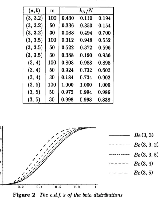
in Table 1. (See also Figure 1.) When $G$ is the c.d.f. of the

beta distributin Be$(3, 3))$ for $(a, b)=(3,3.2)$, (3,3.5), $(3, 4)$, $(3, 5)$ and $N=500$, we have

the values of the approximate power $k_{N}/N$ as in Table 2. (See also Figure 2.)

Table 1Comparison

_of

the approximate power $k_{N}/N$

of

the test in three simulation

results in case

_of

Be(4, 4)

Be$(4, 4)$

Be(4, _4. 2)

—— Be(4, 4. 5) ——- Be$(4, 5)$

Figure 1The

_c.d.f.

’s

_of

the beta distributions

Table 2Comparison

_of

the approimate power $k_{N}/N$

of

the test in three simulation

results in

case

_of

Be(3, 3) Be$(3, 3)$ Be(3, _3. 2) Be(3, _3. 5) —— Be$(3, 4)$ ——- Be$(3, 5)$

Figure 2The

_c.d.f.

’s

_of

the beta distributions

As is

seen

from Table 1, the values of approximate power

are

comparatively stable

except for the

cases

when $(a, b)=(4,4.5)$ and $m=1\mathrm{O}\mathrm{O}$,

which

are

due to the first sample

from the distribution Be$(4, 4)$. Table 2shows asimilar tendency to the result in Table 1.

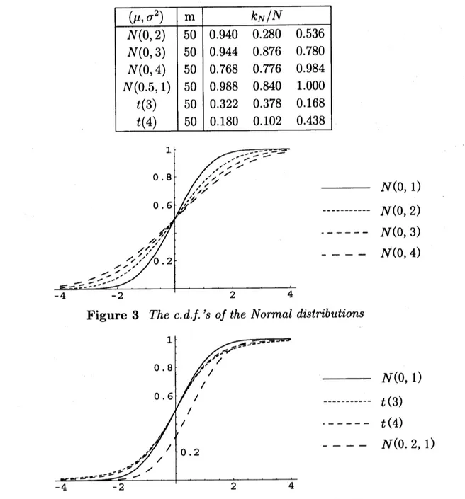
(ii) Let $F$ be the c.d.f. of the standard normal distribution $N(0,1)$ and $G$ the c.d.f. of

$N(\mu, \sigma^{2})$. For $\alpha=0.05$, $(\mu, \sigma^{2})=(0,2)$,$(0, 3)$, $(0, 4)$, (0.5, 1) and $N=500$,

we

have the

values of the approximate power $k_{N}/N$ is three simulation results

as

in Table 3. When

$(\mu, \sigma^{2})=(0,2)$, they

seems

to be unstable.

Table 3Comparison

_of

the approximate power $k_{N}/N$

of

the test in three simulation

results in

case

_of

$N(0,$1)

$N(0, 1)$ $N(0, 2)$

$——$

$N(0, 3)$

$—-$

$N(0, 4)$

Figure 3The

_c.d.f.

’s

_of

the Normal distributions

$N(0,1)$

$t(3)$

—— $t(4)$

——- $N(0.2,1)$

Figure 4The

_c.d.f.

’s

_of

the Normal distributions and t-distribution

3. Remarks

The

tw0-sample problem in

this paper

may be

applied to

the

foUowing

.

Suppose that

adrug is admitted

as

amarketable

one

in

some

countriesafter testingits efficacy bymany

data. When those date

are

available, the problem is how to test the efficacy of the drug

by onlysmalldatain anothercountry. In theproblemthe size of small datais important,

and, according to

our

simulation study, the result

seems

to be comparatively stable for

the size 50, though it

may

depend

on

the population

distribution

and the first sample

from it.

References

Akahira, M. and Takeuchi, K. (1991). Bootstrap

method

and empirical

process. Ann.

Inst.

Statist.

Math., 43,

_297-310.

Birnbaum, Z. W. (1952). _{Numerical tabulation of the distribution of Kolmogorov’s}

statistic for finite sample size. J. Amer. Statist. Assoc, 47, 425-441.

Miller, L. H. (1956). Table of percentage points of Kolmogorov statistics. J.

Amer.

Statist. Assoc, 51, 111-121.

lSuch amedical problemwas brought by Prof. M. Takeuchi ofKitasato Universitytothefirst author