EQUATIONS GOVERNING CONVECTION IN EARTH'S CORE AND THE GEODYNAMO

EQUATIONS

GOVERNING

CONVECTION IN EARTH’S CORE

AND THE GEODYNAMO

PAUL H. ROBERTS

Department

_of

Mathematics, and Institute

_of

Geophysics $\partial$ Planetary Physics,

University

_of

California, $Los$ Angeles,

California

90024

Summary

A general strategy is presented for the study of convection in a turbulent fluidsystem

such as Earth’s core. This strategy is also applicable to systems much less complicated

than Earth’s core, $\mathrm{w}\mathrm{h}\mathrm{i}_{\mathrm{C}}.\mathrm{h}$is a rapidly rotatingmagnetohydrodynamicbody of metallic alloy

that slowly evolves as it cools. These added complicationsmust howeverbe included when the Earth’s magnetic field is explained by dynamo action in the core.

1. Development of a Strategy

This paper is a distillation of a paper with the same title by Braginsky

&Roberts

(1995), which will be referred to as $‘ \mathrm{B}\mathrm{R}$”, and ofa recent paper describing a geodynamo

simulation (Glatzmaier&Roberts, $1996\mathrm{b}$). The latter, which willbe referred to as “$\mathrm{G}\mathrm{R}2$”,

put the BR theory to work. Related simulations (“$\mathrm{G}\mathrm{R}1$”

&‘‘GRIA’’)

are described in

Glatzmaier

&Roberts

($1995\mathrm{a},$ $1995\mathrm{b}$ for simulation $\mathrm{G}\mathrm{R}1;1996\mathrm{a}$ for simulation GRIA).

Figure 1 shows a rough sketch of Earth’s interior, the system considered in this paper.

Fig. 1: A sketch of Earth’s interior

GR1

&GRIA

are Boussinesq simulations that ignore the variation of density, $\rho$,

anelastic model which includes that variation, the assumed structure of Earth’s interior

being guidedbythe PREM model of

Dziewonski&Anderson

(1981). The variation ofcore

structure with depth is described by a parameter $\epsilon_{a}$, which is essentially the difference in

$\rho$ at the inner core boundary

$(” \mathrm{I}\mathrm{C}\mathrm{B}")$ and the core-mantleboundary $(” \mathrm{C}\mathrm{M}\mathrm{B}")$ divided by

the mean density, and is of order 0.1. It is the smallness of this parameter that makes

it reasonable to represent the core by a Boussinesq model, though doubtless the anelastic

model is more satisfactory.

Convection in the core is so vigorous that all extensive quantities, such as the specific

entropy, $S$, are very well mixed. To measure this effect, we may introduce a dimensionless

parameter, $\epsilon_{c}=S_{c}/S_{a}$, where $S_{\mathrm{c}}=S-S_{a}$ is the departure of $S$ from its value, $S_{a}$, in

the well-mixed state; it is found that $\epsilon_{\mathrm{c}}\sim 10^{-8}$

.

As is usual in convection theory, we

describe convection in two steps: first we select a convenient reference state, and second

we study departures from that reference state associated with convection. It is clear that

a convenient reference state is the well-mixedstate, that has uniformentropy for anelastic

models and uniform temperature for Boussinesq models.

GRI&GRIA

are driven steadily

by a specified heat flux at the ICB; GR2 is drivenby heat conducted out of the core into

the mantle across the CMB. The reference state of GR2 therefore changes secularly on a

geological timescale, $t_{a}$, as the Earth cools, whereas the reference states of

GRI&GRIA

are steady.

A further complication, in the case of the Earth, is that bouyancy is provided not

only thermally but also chemically, by differences in composition. Though the core is “an

uncertain mixture of all the elements”, there seems to be little doubt that it is abundent

in iron. There is general agreement that the fluid outer core $(” \mathrm{F}\mathrm{O}\mathrm{C}")$ is significantly less

dense than iron would be at core pressures, and that alloying elements must be present.

There is no consensus on what the alloying elements are, or even what the predominant

light constituent is. From a theoretical point of view, the basic physics is satisfied by assuming the simplest possible case, in which there is only one alloying element its mass

fraction being $\xi$. This too is well mixed by the convection, so that $\xi_{a}$ is almost uniform

in space, though dependent on $t_{a}$

.

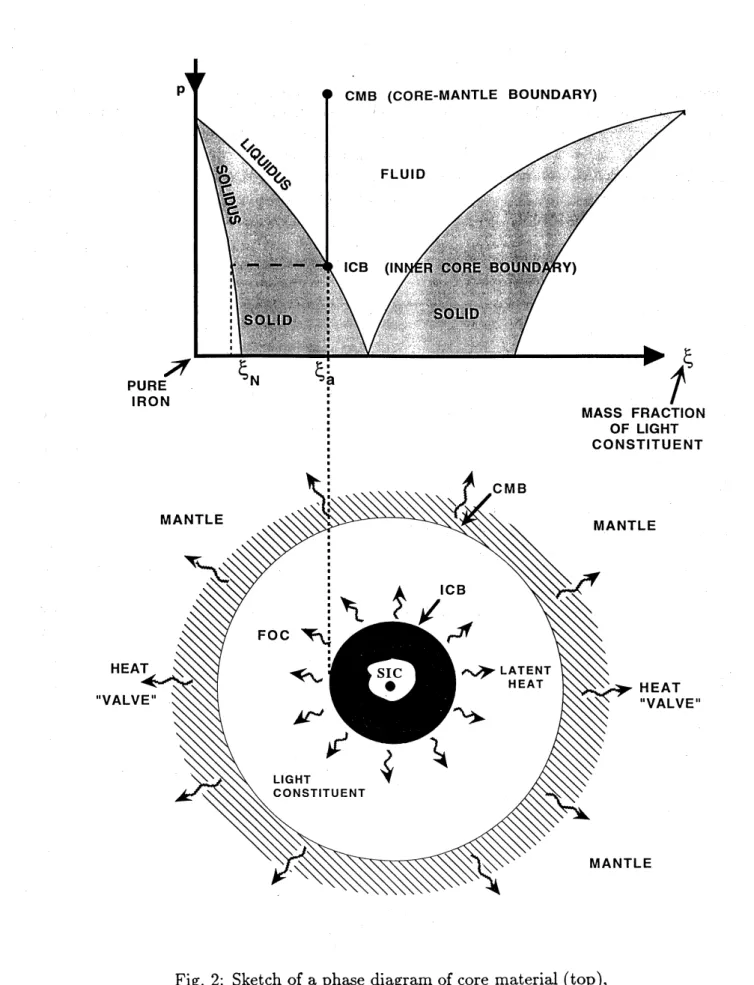
Seismological models of the Earth’s interior show that

the density of the solid inner core $(” \mathrm{S}\mathrm{I}\mathrm{C}")$is closer to that of pure iron than is that of the

FOC. There is a density jump across the ICB of about 0.$55\mathrm{g}\mathrm{m}/\mathrm{c}\mathrm{c}$, presumably because

the value $\xi_{N}$ of $\xi$ at the top of the SIC is less than $\xi_{a}$. This is naturally the case if, as is

now believed, the ICB is afreezing interface. A simple phase diagram which would lead to

such a conclusion is shown in the upper part of Figure 2. A phase diagram usually shows the solidus and liquidus of a material as curves in $\xi T$-space. This is because they are

generally discussed in contexts where variations in pressure,$p$, are unimportant. Inreality

the liquidus and solidus depend on the thermodynamic state of thematerial. They should therefore appear as surfaces in three-dimensions. The traditional diagrams showing them

as curvesare merely intersectionsof these surfaces with the appropriate$\mathrm{c}\mathrm{o}\mathrm{n}\mathrm{s}\mathrm{t}\mathrm{a}\mathrm{n}\mathrm{t}-p$ plane.

In thecontext of the core it is appropriate to plot the solidus and liquidus in$\xi pS$-space and

to project them onto the plane $S=S_{a}$

.

Thisis the way they are shown in Figure 2, where

we focus attention on the left-hand solidus and liquidus only. On descending through the FOC from the CMB, we eventually encounter the ICB, where the pressure is such

Fig. 2: Sketch of a phase diagram of core material (top),

and light constituent as it does so. These sources of buoyancy establish core convection that stirs thefluid, making$S_{a}$ and$\xi_{a}$ almostuniform,andgeneratingthe Earth’s magnetic

field by dynamo action. GR2 includes both these sources;

GRI&IA

recognizes thermal

buoyancy alone. It should perhaps be emphasized that, although it is necessary in GR2

to include both sources of buoyancy and to allow the reference state to evolve in time, these complications arenot essential in other applications (and are not in fact includedin

GR1

_&GRIA).

The theory we describe below, which contains a few novelties, therefore

has wider applications. As in many other applications of convection theory, motions in Earth’s core are on many length and time scales. That this must be the case is clear

when we consider quantities such as the P\’eclet number, $\overline{P}=\overline{VL}/\kappa^{T}$, and the Schmidt

number, $\overline{S}--\overline{VL}/\kappa^{\xi}$, of the macroscale defined

$\cdot$

by a characteristic macroscale velocity $\overline{V}$

and length $\overline{L}$ and by typical

molecular diffusivities $\kappa^{T}$ and $\kappa^{\xi}$

of heat and composition. Taking$\overline{V}=10^{-4}\mathrm{m}/\mathrm{s}$and$\overline{L}=10^{6}\mathrm{m}$, we find that$\overline{P}\sim 10^{7}$ and$\overline{S}\sim 10^{12}$

.

This shows that

molecular transport of heat and composition is almost totally ineffective on the microscale. It is also true of the momentum transport as measured by the kinetic Reynolds number,

$\overline{R}=\overline{VL}/\nu^{m}\sim 10^{5}$, where $\nu^{m}$ is the molecular kinematic viscosity. It is clear that, to

transport heat, composition and momentum on the macroscale, the core has to develop small scale motions (turbulence).

The incorporation of turbulence into the theory is an unavoidable complication that has to be overcomein a physically consistent way. We adopt the simplest possible model: a local turbulence theory in which a field such as $S_{\mathrm{c}}$ is divided into a macroscale part, $\overline{S}$,

and a microscale part, $S’,$ $\mathrm{e}.\mathrm{g}^{1}.$, We then develop expressions for the macroscale fluxes of

entropy, composition and momentum at position $\mathrm{x}$ and time $t$ created by the turbulence.

In a local theory, these depend on the macroscale properties of the system, but only at

the same $\mathrm{x}$ and $t$. The evaluation of these fluxes requires separate and detailed study; see

Appendix $\mathrm{C}$ of$\mathrm{B}\mathrm{R}$, the paper of Braginsky&Meytlis (1990), and the discussion below.

The steps required to develop a workable theory of core convection and the geodynamo are now apparent; they are summarized in Table $0$ and by the following supplementary

remarks. Concerning step 2 of the table, the rearrangement of mass inherent in a cooling Earth can only be brought about by motions of order $V_{a}\sim 10^{-12}\mathrm{m}/\mathrm{s}\sim\epsilon_{c}V_{c}$, which is

so small that the momentum equation reduces to an expression of hydrostatic balance. Concerning step 3, $\epsilon_{c}$ is so small that it is possible to linearize the thermodynamics about

the well mixed state of uniform entropy and composition, though all other nonlinearities must be retained. We should also point out that seismic waves cross Earth’s core in about

10 minutes. Not only is such a smalltime scale irrelevant to the phenomenon under study, but also to include it would require such short time steps in a numerical simulation that

1 _{The overbar on}$\overline{S}$ denotes anaverage

over turbulent ensembles and $S’$ is the

superim-posedturbulentpartof$S$. Thisnotation is often used in mean field electrodynamics; see for

example Krause&R\"adler (1980). Itis different from that ofBRwhowrote$S_{c}=\langle S_{c}\rangle^{t\mathrm{t}}+^{s}$.

They did this to avoidapossible ambiguity: an overbar is often used in geomagnetic theory to signify the axisymmetric part of a field, i.e., an average over longitude; a prime then signifies the asymmetric part of the field.

Table $0$:

STRATEGY:

Development of Basic Convection Equations

it would render it totally

impractical2.

We therefore adopt the anelastic approximation in which $\partial\rho_{c}/\partial t$ is neglected in the continuity equation. This “filters out” sound waves. Once

2 _{This statement, though true for Earth’s core, is not universally applicable to all}

convective dyanamos. For example, Kageyama et al. (1995) consider convectionin ahighly

compressible body of fluid. If their model were scaled to core conditions,soundwouldtake decades to cross the core. Under such circumstances it would be incorrect to replace the continuity equation by the anelastic equation, and in fact they did not do so.

thefinal anelastic equations have been derived (see step $6\mathrm{A}$), areduction to a

Boussinesq-type theory is possible (step $6\mathrm{B}$). This is described in

\S 8

of $\mathrm{B}\mathrm{R}$; an even simpler form

of Boussinesq convection is used in the GR1 and GRIA simulations. The anelastic and

Boussinesq-like theories haveinterestingthermodynamic implicationsconcerning the ther-modynamic efficiency of convective systems, regarded as heat engines (step $7\mathrm{A}\mathrm{B}$). These

are discussed in

\S 7

of $\mathrm{B}\mathrm{R}$, but will not be described here. One further point should be

mentioned. The gravity defining the reference state is the effective gravity, $\mathrm{g}_{\mathrm{e}}$,whichdiffers

from Newtonian gravity, $\mathrm{g}$, by the centrifugal acceleration due to Earth’s rotation. The

whole Earth (including the ICB and CMB) is therefore slightly flattened. The significance of this effect is measured by a further dimensionless parameter, $\epsilon_{\Omega}=\Omega^{2}\overline{L}/\overline{g}\sim 10^{-3}$, where

$\Omega$ is the angular velocity of Earth and $\overline{g}$ is a characteristic gravitational acceleration. It

is clear that the effect is not large, but to include it would add severe complications to

the theory without any compensating enlightenment. We shall therefore later set $\epsilon_{\Omega}\equiv 0$,

though we shall retain the Coriolis force. The steps leading from $6\mathrm{A}$ to $6\mathrm{B}$ may be found

in BR and are not repeated in the present paper. 2. The Strategy in Greater Detail

The arguments that BR employed to complete the strategy set out in Table $0$ are

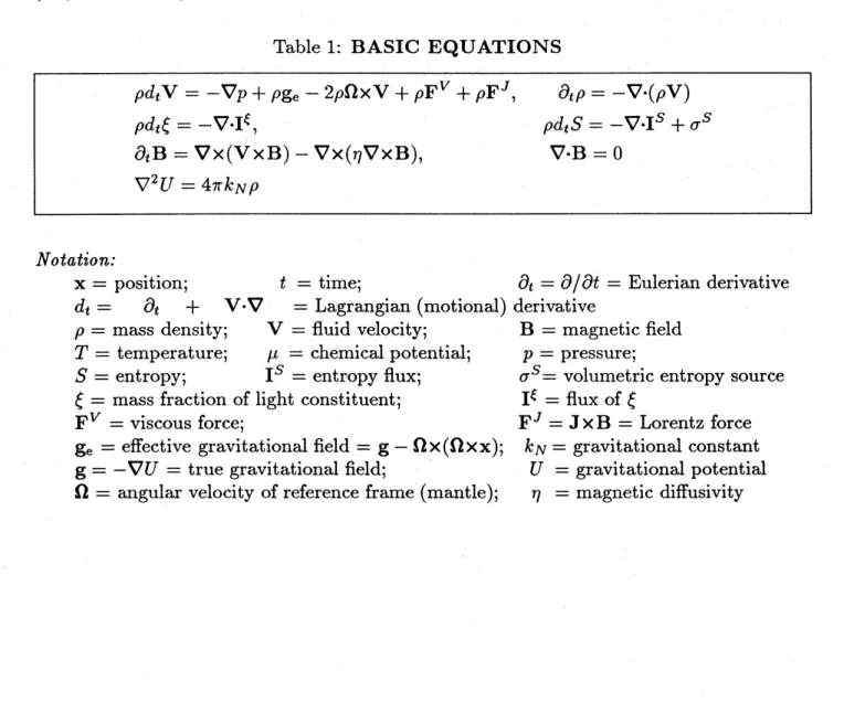
fully set out in BR and will therefore be described only briefly here. The basic equations (step 1 in Table$0$) aresummarizedin Table 1, which also containsashort table ofnotation.

Table 1: BASIC EQUATIONS

$\rho d_{t}\mathrm{V}=-\nabla p+\rho \mathrm{g}_{\mathrm{e}}-2\rho\Omega\cross \mathrm{V}+\rho \mathrm{F}^{V}+\rho \mathrm{F}^{J}$ , $\partial_{t}\rho=-\nabla\cdot(\rho \mathrm{V})$ $\rho d_{t}\xi=-\nabla\cdot \mathrm{I}^{\xi}$, $\rho d_{t}S=-\nabla\cdot \mathrm{I}s+\sigma^{s}$

$\partial_{t}\mathrm{B}=\nabla\cross(\mathrm{V}\mathrm{x}\mathrm{B})-\nabla\cross(\eta\nabla\cross \mathrm{B})$ , $\nabla\cdot \mathrm{B}=0$

$\nabla^{2}U=4Tk_{N}\rho$

Notation:

$\mathrm{x}=\mathrm{p}_{\mathrm{o}\mathrm{S}\mathrm{i}\mathrm{t}\mathrm{i}\mathrm{o}\mathrm{n}}$; $t=\mathrm{t}\mathrm{i}\mathrm{m}\mathrm{e}$; $\partial_{t}=\partial/\partial t=\mathrm{E}\mathrm{u}\mathrm{l}\mathrm{e}\mathrm{r}\mathrm{i}\mathrm{a}\mathrm{n}$ derivative

$d_{t}=$ $\partial_{t}$ _$+$ $\mathrm{V}\cdot\nabla$

$=\mathrm{L}\mathrm{a}\mathrm{g}\mathrm{r}\mathrm{a}\mathrm{n}\mathrm{g}\mathrm{i}\mathrm{a}\mathrm{n}$ (motional) derivative $\rho=\mathrm{m}\mathrm{a}\mathrm{s}\mathrm{s}$ density;

$\mathrm{V}=\mathrm{f}\mathrm{l}\mathrm{u}\mathrm{i}\mathrm{d}$ velocity; $\mathrm{B}=\mathrm{m}\mathrm{a}\mathrm{g}\mathrm{n}\mathrm{e}\mathrm{t}\mathrm{i}\mathrm{C}$field $T=\mathrm{t}\mathrm{e}\mathrm{m}\mathrm{p}\mathrm{e}\mathrm{r}\mathrm{a}\mathrm{t}\mathrm{u}\mathrm{r}\mathrm{e}$; $\mu=\mathrm{c}\mathrm{h}\mathrm{e}\mathrm{m}\mathrm{i}\mathrm{c}\mathrm{a}\mathrm{l}$potential;

$p=\mathrm{P}^{\mathrm{r}\mathrm{e}\mathrm{S}\mathrm{s}\mathrm{u}\mathrm{r}\mathrm{e}}$;

$S=\mathrm{e}\mathrm{n}\mathrm{t}\mathrm{r}\mathrm{o}\mathrm{p}\mathrm{y}$; $\mathrm{I}^{S}=\mathrm{e}\mathrm{n}\mathrm{t}\mathrm{r}\mathrm{o}\mathrm{p}\mathrm{y}$ flux; $\sigma^{S}=\mathrm{v}\mathrm{o}\mathrm{l}\mathrm{u}\mathrm{m}\mathrm{e}\mathrm{t}\mathrm{r}\mathrm{i}\mathrm{c}$entropy

source

$\xi=\mathrm{m}\mathrm{a}\mathrm{s}\mathrm{s}$fraction oflight constituent;

$\mathrm{I}^{\xi}=\mathrm{f}\mathrm{l}\mathrm{u}\mathrm{x}$ of $\xi$

$\mathrm{F}^{V}=\mathrm{v}\mathrm{i}\mathrm{s}\mathrm{C}\mathrm{o}\mathrm{u}\mathrm{s}$ force; $\mathrm{F}^{J}=\mathrm{J}\cross \mathrm{B}=\mathrm{L}\mathrm{o}\mathrm{r}\mathrm{e}\mathrm{n}\mathrm{t}\mathrm{Z}$force $\mathrm{g}_{\mathrm{e}}=\mathrm{e}\mathrm{f}\mathrm{f}\mathrm{e}\mathrm{c}\mathrm{t}\mathrm{i}\mathrm{V}\mathrm{e}$gravitational field $=\mathrm{g}^{-\Omega\cross}(\Omega\cross \mathrm{x})$; $k_{N}=\mathrm{g}\mathrm{r}\mathrm{a}\mathrm{v}\mathrm{i}\mathrm{t}\mathrm{a}\mathrm{t}\mathrm{i}_{\mathrm{o}\mathrm{n}\mathrm{a}1}$constant

$\mathrm{g}=-\nabla U--\mathrm{t}\mathrm{r}\mathrm{u}\mathrm{e}$gravitational field; $U=\mathrm{g}\mathrm{r}\mathrm{a}\mathrm{v}\mathrm{i}\mathrm{t}\mathrm{a}\mathrm{t}\mathrm{i}_{\mathrm{o}\mathrm{n}\mathrm{a}1}$potential $\Omega=\mathrm{a}\mathrm{n}\mathrm{g}\mathrm{u}\mathrm{l}\mathrm{a}\mathrm{r}$velocity of reference frame (mantle); $\eta=\mathrm{m}\mathrm{a}\mathrm{g}\mathrm{n}\mathrm{e}\mathrm{t}\mathrm{i}_{\mathrm{C}}$diffusivity

The reference state (step 2) is described in Table 2. Of particular interest here is the introduction of a generalized potential II such that $\Gamma \mathrm{I}_{a}$ is, like $S_{a}$ and $\xi_{a}$, uniform in

the reference state. In this table, $us$ is the speed of sound and $c_{p}$ is the specific heat at

constant pressure. All such quantities are evaluated in the reference state.

Table 2: REFERENCE STATE

Well-mixed State in (approximate) Hydrostatic Equilibrium:

$\nabla\xi_{a}=0$, V$S_{a}=0$

$\rho_{a}^{-1}\nabla p_{a}=-\nabla U_{\mathrm{e}}a\equiv \mathrm{g}_{\mathrm{e}a}$, $\nabla^{2}U\mathrm{e}a=4\pi kN\rho_{a}-2\Omega^{2}$

$\nabla\cdot(\rho_{a}\mathrm{V}_{a})=-\dot{\rho}_{a}$, $\mathrm{B}_{a}=0$

Variables are functions of$\mathrm{x}$ and of the slow time scale, $t_{a}$; $\xi$ and $S$ are independentof $\mathrm{x}$.

So is II $=\epsilon^{H}+U$, where $\epsilon^{H}=\mathrm{e}\mathrm{n}\mathrm{t}\mathrm{h}\mathrm{a}\mathrm{l}\mathrm{p}\mathrm{y}/\mathrm{u}\mathrm{n}\mathrm{i}\mathrm{t}$ mass. Hydrostatic $equilibrium\Rightarrow$

$\nabla\Pi_{a}=0$

Elementary Consequences:

$\rho_{a}=\rho$($p_{a},$

s

,$\xi_{a}$), $T_{a}=T$(

$pa’$

sa’

$\xi a$), _{$\mu_{a}=\mu$}($p_{a’}$

s

,$\xi_{a}$)

and

$\rho_{a}^{-1}\nabla\rho_{a}=\mathrm{g}\mathrm{e}a/u_{S}^{2}$, $\nabla\mu_{a}=\alpha\epsilon_{\mathrm{g}_{\mathrm{e}a}}$, $\nabla T_{a}=\alpha s\mathrm{g}\mathrm{e}a$

where

$\alpha^{\xi}=-\frac{1}{\rho}(\frac{\partial p}{\partial\xi})_{p,S}$, $\alpha^{S}=-\frac{1}{\rho}(\frac{\partial\rho}{\partial S})_{P},\xi=\frac{\alpha T}{c_{p}}$

More familiar form:

$\tau_{a}^{-1}\nabla Ta=\gamma \mathrm{g}_{\mathrm{e}a}/u_{S}^{2}$, $\gamma=\alpha u_{S}^{2}/c_{p}=\mathrm{t}\mathrm{h}\mathrm{e}$ Gr\"uneisen constant

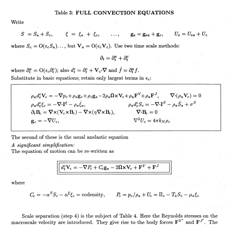
The basic anelastic equations (step 3) are set out in Table 3, and a remarkable sim-plification discovered by BR is briefly set out. This consists of a new way of writing the

anelastic momentum equation that has two great advantages over the primative form of that equation. First, it obviates the need to calculate the perturbation, $\mathrm{g}_{c}$, in $\mathrm{g}$ created

by the perturbation, $\rho_{c}$, in density. If$\mathrm{g}_{c}$ is deemed to be interesting, it can be evaluated

after the main part of the calculation has been completed. Second, it is clear on physical grounds that densityvariations produced by pressure variations, $p_{c}$, will not drive

convec-tion. The simplification allows that part of $\rho_{c}$ to be split off from $\rho_{c}$ and absorbed into

the gradient term, so leaving the remaining variations in $\rho_{c}$ due to changes in entropy and

composition to be included in the “

Table 3: FULL CONVECTION EQUATIONS Write

$S=S_{a}+S_{c}$, $\xi=\xi_{a}+\xi_{c}$,

...

,

$\mathrm{g}_{\mathrm{e}}=\mathrm{g}_{\mathrm{e}a}+\mathrm{g}_{c}$, $U_{\mathrm{e}}=U_{\mathrm{e}a}+U_{\mathrm{C}}$

where $S_{c}=\mathrm{O}(\epsilon_{c}s_{a})\ldots$ , but $\mathrm{V}_{a}=\mathrm{O}(\epsilon_{c}\mathrm{V}_{c})$

.

Use two time scale methods: $\partial_{t}=\partial^{a}+t\partial^{c}t$

where $\partial_{t}^{a}=\mathrm{O}(\epsilon_{ct}\partial^{C})$; also $d_{t}^{c}=\partial_{t}^{c}+\mathrm{V}_{c}\cdot\nabla$ and $\dot{f}=\partial_{t}^{a}f$

.

Substitute in basic equations; retain only largest terms in $\epsilon_{c}$:

.

$p_{a}d_{t}^{c}\mathrm{V}_{c}=-\nabla p_{c}+\rho a\mathrm{g}c+\rho C\mathrm{g}_{a}-2pa\Omega \mathrm{X}\mathrm{v}\mathbb{C}+\rho_{a}\mathrm{F}^{V}+\rho a\mathrm{F}^{J}$, $\nabla\cdot(\rho_{a}\mathrm{V}_{c})=0$

$\rho_{a}d_{t}^{c}\xi_{\mathrm{C}}=-\nabla\cdot \mathrm{I}^{\xi}-p_{a}\dot{\xi}_{a}$, $\rho_{a}d_{t}^{c}S_{c}=-\nabla\cdot \mathrm{I}^{S}-\rho_{a}\dot{S}_{a}+\sigma^{S}$

$\partial_{t}\mathrm{B}_{c}=\nabla\cross(\mathrm{V}_{c}\cross \mathrm{B}_{c})-\nabla\cross(\eta\nabla \mathrm{X}\mathrm{B}_{c})$ , $\nabla\cdot \mathrm{B}_{c}=0$

$\mathrm{g}_{c}=-\nabla U_{C}$, $\nabla^{2}U_{\mathrm{c}}=4\pi k_{N}\rho_{c}$

The second of these is the usual anelastic equation A significant simplification:

The equation of motion can be $\mathrm{r}\mathrm{e}$-written as

$d_{t}^{c}\mathrm{v}_{\mathrm{c}}=-\nabla P_{c}+C_{c}\mathrm{g}_{a}-2\Omega \mathrm{X}\mathrm{v}_{c}+\mathrm{F}^{V}+\mathrm{F}^{J}$

where

$C_{c}=-\alpha^{s_{S_{\mathrm{C}^{-}}}\xi}\alpha\xi_{c}=\mathrm{c}\mathrm{o}\mathrm{d}\mathrm{e}\mathrm{n}\mathrm{S}\mathrm{i}\mathrm{t}\mathrm{y}$, _{$P_{c}=p_{c}/\rho_{a}+U_{c}=\Pi_{c}-\tau as\mathrm{C}^{-\mu\xi}a\mathrm{C}$}

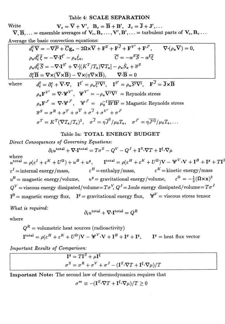
Scale separation (step 4) is the subject of Table 4. Here the Reynolds stresses on the

macroscale velocity are introduced. They give rise to the body forces $\mathrm{F}^{V’}$ and $\mathrm{F}^{J’}$

.

The viscous force associated with the mean motion is $\mathrm{d}\mathrm{e}\mathrm{n}\dot{\mathrm{o}}\mathrm{t}\mathrm{e}\mathrm{d}$by $\mathrm{F}^{\overline{\nu}}$

.

It $\mathrm{a}\mathrm{p}\dot{\mathrm{p}}$ears

to be negligible in the geophysical application except in boundary layers. The mean Lorentz force, $\mathrm{F}^{\overline{J}}$

, is

however very significant. The mean fluxes, $\mathrm{I}^{S’}$

and$\mathrm{I}^{\xi}’$

, of entropy and composition created by the turbulence are also important.. It may be seen in Table 4 that the transport of

heat “down the adiabat” ofthe reference state and the associated entropy production $\sigma^{T}$

are both included. These are not negligible in the Earth’s core.

In preparation for step 5, the discussion of aspects of local turbulence theory (Table

$5\mathrm{c})$, Table $5\mathrm{a}$ provides a reminder of the basic theory underlying the general expressions

for entropy flux and compositional flux. This leads to a form for the associated entropy production, $\sigma^{m}$

,

and this has to be non-negative by the second law of thermodynamics.

Table 4: SCALE SEPARATION Write $\mathrm{V}_{c}=\overline{\mathrm{V}}+\mathrm{V}’$, $\mathrm{B}_{c}=\overline{\mathrm{B}}+\mathrm{B}’$, $\mathrm{J}_{c}=\overline{\mathrm{J}}+\mathrm{J}’,$

$\ldots$

$\overline{\mathrm{V}},\overline{\mathrm{B}},$$\ldots=\mathrm{e}\mathrm{n}\mathrm{s}\mathrm{e}\mathrm{m}\mathrm{b}\mathrm{l}\mathrm{e}$ averages of $\mathrm{V}_{\mathrm{c}},$$\mathrm{B}_{c}\ldots,\mathrm{V}’,$$\mathrm{B}’,$$\ldots=\mathrm{t}\mathrm{u}\mathrm{r}\mathrm{b}\mathrm{u}\mathrm{l}\mathrm{e}\mathrm{n}\mathrm{t}$ parts of $\mathrm{V}_{c},$$\mathrm{B}_{c}\ldots$

Average the basic convection equations:

$d_{t}^{\overline{c}}\overline{\mathrm{V}}=-\overline{\nabla P}+^{\overline{c}-2}\mathrm{g}_{a}\Omega\cross\overline{\mathrm{V}}+\mathrm{F}^{\overline{\nu}}+\mathrm{F}^{\overline{J}}+\mathrm{F}^{V’}+\mathrm{F}^{J’}$ , $\nabla\cdot(\rho_{a}\overline{\mathrm{V}})=0$, $\rho_{a}d_{t}^{\overline{\mathrm{c}}}\overline{\xi}=-\nabla\cdot \mathrm{I}^{\xi’}-\rho_{a}\dot{\xi}_{a}$, $\overline{C}=-\alpha\overline{S}S-\alpha\overline{\xi}\xi$

$\rho_{a}d_{t}^{\overline{c}}\overline{S}=-\nabla\cdot \mathrm{I}^{S’}+\nabla\cdot[(Ic^{T}/Ta)\nabla T_{a}]-\rho_{a}\dot{s}_{a}+\overline{\sigma}^{S}$ $\partial_{t}^{c}\overline{\mathrm{B}}=\nabla\cross(\overline{\mathrm{V}}\mathrm{X}\overline{\mathrm{B}})-\nabla\cross(\eta\nabla\cross\overline{\mathrm{B}})$, $\nabla\cdot\overline{\mathrm{B}}=0$

where $d_{t}^{\overline{\mathrm{C}}}=\partial_{t}c+\overline{\mathrm{V}}\cdot\nabla$, $\mathrm{I}^{\xi’}=\rho_{a}\overline{\xi’\mathrm{V}’}$, $\mathrm{I}^{S’}=\rho_{a}\overline{S’\mathrm{V}’}$,

$\mathrm{F}^{\overline{J}}=\overline{\mathrm{J}}\cross\overline{\mathrm{B}}$

$\rho_{a}\mathrm{F}^{V’}=\nabla\cdot 7^{V’}$,

7

$V’=-\rho_{a}\overline{\mathrm{V}’\mathrm{v}\prime}=\mathrm{R}\mathrm{e}\mathrm{y}\mathrm{n}\mathrm{o}\mathrm{l}\mathrm{d}_{\mathrm{S}}$stress

$\rho_{a}\mathrm{F}^{J’}=\nabla\cdot\forall^{J’}$ , $\tau^{J’}=$ $\mu_{0}^{-1}\overline{\mathrm{B}’\mathrm{B}’}=\mathrm{M}\mathrm{a}\mathrm{g}\mathrm{n}\mathrm{e}\mathrm{t}\mathrm{i}\mathrm{c}$Reynolds stress

$\overline{\sigma}=\sigma+\sigma^{\tau}+sR\sigma+\overline{V}\overline{J}\sigma+\sigma^{V’}+\sigma^{J’}$

$\sigma^{T}=K\tau(\nabla\tau_{a}/\tau_{a})^{2}$, $\sigma^{\overline{J}}=\eta\overline{J}^{2}/\mu 0^{T_{a}}$, $\sigma^{J’}=\eta\overline{J^{\prime 2}}/\mu 0^{T_{a}},$ $\ldots$

Table $5\mathrm{a}$: TOTAL ENERGY BUDGET

Direct Consequences

_of

Governing Equations:

$\partial_{t}u^{\mathrm{t}\circ \mathrm{t}}+\mathrm{a}1\nabla\cdot \mathrm{I}\mathrm{t}_{0}\mathrm{t}\mathrm{a}1=^{\tau_{\sigma}}s_{-Q-}VQ^{J}+\mathrm{I}^{s_{\nabla T}}\cdot+\mathrm{I}\epsilon.\nabla\mu$

where

$u^{\mathrm{t}\circ \mathrm{t}\mathrm{a}1}=\rho(\mathcal{E}^{I}+6^{K\Omega}+U)+u+uBg$ , $\mathrm{I}^{\mathrm{t}\mathrm{o}\mathrm{t}\mathrm{a}}1(=\rho\epsilon+\epsilon+U^{\Omega}HK)\mathrm{V}-\varphi^{V}.\mathrm{v}+\mathrm{I}^{B}+\mathrm{I}g+^{\tau}\mathrm{I}s_{+}\mu \mathrm{I}$

$\epsilon^{I}=\mathrm{i}\mathrm{n}\mathrm{t}\mathrm{e}\mathrm{r}\mathrm{n}\mathrm{a}\mathrm{l}\mathrm{e}\mathrm{n}\mathrm{e}\mathrm{r}\mathrm{g}\mathrm{y}/\mathrm{m}\mathrm{a}\mathrm{s}\mathrm{s}$, $\epsilon^{H}=\mathrm{e}\mathrm{n}\mathrm{t}\mathrm{h}\mathrm{a}\mathrm{l}\mathrm{p}\mathrm{y}/\mathrm{m}\mathrm{a}\mathrm{s}\mathrm{s}$, $\epsilon^{K}=\mathrm{k}\mathrm{i}\mathrm{n}\mathrm{e}\mathrm{t}\mathrm{i}\mathrm{c}\mathrm{e}\mathrm{n}\mathrm{e}\mathrm{r}\mathrm{g}\mathrm{y}/\mathrm{m}\mathrm{a}\mathrm{s}\mathrm{s}$ $u^{B}=\mathrm{m}\mathrm{a}\mathrm{g}\mathrm{n}\mathrm{e}\mathrm{t}\mathrm{i}_{\mathrm{C}}\mathrm{e}\mathrm{n}\mathrm{e}\mathrm{r}\mathrm{g}\mathrm{y}/\mathrm{v}\mathrm{o}\mathrm{l}\mathrm{u}\mathrm{m}\mathrm{e}$, $u^{g}=\mathrm{g}\mathrm{r}\mathrm{a}\mathrm{v}\mathrm{i}\mathrm{t}\mathrm{a}\mathrm{t}\mathrm{i}\mathrm{o}\mathrm{n}\mathrm{a}\mathrm{l}\mathrm{e}\mathrm{n}\mathrm{e}\mathrm{r}\mathrm{g}\mathrm{y}/\mathrm{v}\mathrm{o}\mathrm{l}\mathrm{u}\mathrm{m}\mathrm{e}$, $\epsilon^{\Omega}=-\frac{1}{2}(\Omega\cross \mathrm{x})^{2}$ $Q^{V}=\mathrm{v}\mathrm{i}_{\mathrm{S}}\mathrm{C}\mathrm{o}\mathrm{u}\mathrm{S}$ energy $\mathrm{d}\mathrm{i}_{\mathrm{S}}\mathrm{s}\mathrm{i}_{\mathrm{P}^{\mathrm{a}\mathrm{t}\mathrm{d}}/0}\mathrm{e}\mathrm{V}1\mathrm{u}\mathrm{m}\mathrm{e}=T\sigma,$$QVJ=\mathrm{J}\mathrm{o}\mathrm{u}\mathrm{l}\mathrm{e}$energy

$\mathrm{d}\mathrm{i}_{\mathrm{S}}\mathrm{s}\mathrm{i}\mathrm{p}\mathrm{a}\mathrm{t}\mathrm{e}\mathrm{d}/\mathrm{v}\mathrm{o}\mathrm{l}\mathrm{u}\mathrm{m}\mathrm{e}=T\sigma^{J}$

$\mathrm{I}^{B}=\mathrm{m}\mathrm{a}\mathrm{g}\mathrm{n}\mathrm{e}\mathrm{t}\mathrm{i}\mathrm{c}$ energy flux, $\mathrm{I}^{g}=\mathrm{g}\mathrm{r}\mathrm{a}\mathrm{v}\mathrm{i}\mathrm{t}\mathrm{a}\mathrm{t}\mathrm{i}\mathrm{o}\mathrm{n}\mathrm{a}\mathrm{l}$energy flux,

$7^{V}=\mathrm{v}\mathrm{i}_{\mathrm{S}}\mathrm{C}\mathrm{o}\mathrm{u}\mathrm{S}$ stress tensor What is required:

$\partial_{t}u^{\mathrm{t}\circ \mathrm{t}\mathrm{a}10\iota \mathrm{a}}+\nabla\cdot \mathrm{I}\mathrm{t}1Q^{R}=$

where

$Q^{R}=\mathrm{v}\mathrm{o}\mathrm{l}\mathrm{u}\mathrm{m}\mathrm{e}\mathrm{t}\mathrm{r}\mathrm{i}_{\mathrm{C}}$heat sources (radioactivity)

$\mathrm{I}^{\mathrm{t}\mathrm{o}\mathrm{t}\mathrm{a}1}=\rho(\epsilon H+\epsilon^{K}+U^{\Omega})\mathrm{V}-\mathrm{w}^{V}\cdot \mathrm{v}+\mathrm{I}^{B}+\mathrm{I}^{g}+\mathrm{I}^{q}$, $\mathrm{I}^{q}=\mathrm{h}\mathrm{e}\mathrm{a}\mathrm{t}$ flux vector

Important Results

_of

Comparison:

$\mathrm{I}^{q}=T\mathrm{I}+\mu \mathrm{I}^{\xi}$

$\sigma^{S}=\sigma^{R}+\sigma+\sigma-VJ(\mathrm{I}s.\nabla\tau+\mathrm{I}\epsilon.\nabla\mu)/T$

Important Note: The second law of thermodynamics requires that

In Table $5\mathrm{b}$, we provide a reminder of how this is achieved when molecular transport is

solely responsible for the fluxes of heat and composition. A more detailed account ofthis

topic may be found in the text of Landau

&Lifshitz

(1987). The corresponding local turbulence theory is given in Table $5\mathrm{c}$

.

This employs the Reynolds ansatz, and leads to

an expression for the macroscale entropy production $\sigma^{t}$ created by the macroscale fluxes

I$S’$

and $\mathrm{I}^{\xi’}$

generated by the turbulence. This expression is new and leads to values of $\sigma^{t}$

that, while not as large as some other sources of entropy, are significant in the application

of the theory to $\mathrm{G}\mathrm{R}2$

.

The expression for $\sigma^{t}$ is negative inany domain where the reference

state is stably stratified. That is not surprising since, according to local theory, turbulence cannot exist where the stratification is bottom heavy; penetration of turbulence from adjacent turbulent regions is excluded in a local theory. In such conditions therefore $\sigma^{t}\equiv 0$ and only the contribution, $\sigma^{m}$, made by molecular

fluxes to entropy production is present. When $\sigma^{t}>0$ however, it normally greatly

exceeds $\sigma^{m}$, and the neglect of the latter then results in only a very minor error.

Table $5\mathrm{b}$: MOLECULAR DIFFUSION

Question: Why is $\sigma^{m}\equiv-(\mathrm{I}^{s_{\nabla T}}\cdot+\mathrm{I}^{\xi}\cdot\nabla\mu)/T\geq 0$ at the molecular level?

Answer: (cf. e.g., Landau&Lifschitz, 1987)

Use $p,$ $T$ and $\mu$ as independent variables and suppose that

$\mathrm{I}\epsilon=-\alpha’\nabla\mu-\beta^{;}\nabla T-\epsilon’\nabla p$, $\mathrm{I}^{S}=-\delta’\nabla\mu-\gamma\nabla’\tau-\zeta’\nabla p$

We require that, for independent $\nabla\mu,$ $\nabla T,$ $\nabla p$,

$\tau_{\sigma^{m}=\alpha}’(\nabla\mu)^{2}+\gamma’(\nabla T)2+(\beta/\delta’)+\nabla\mu\cdot\nabla T+\epsilon^{;}\nabla p\cdot\nabla\mu+\zeta’\nabla p\cdot\nabla T\geq 0$

$\Rightarrow$

$\alpha’\geq 0$, $\gamma’\geq 0$, $\epsilon’=\zeta’=0$, $(\beta’+\delta’)^{2}\leq 4\alpha’\gamma’$

Onsager $\mathrm{r}\mathrm{e}\mathrm{c}\mathrm{i}\mathrm{p}\mathrm{r}\mathrm{o}\mathrm{C}\mathrm{i}\mathrm{t}\mathrm{y}\Rightarrow$ $\delta’=\beta’$.

Final result:

$\mathrm{I}^{\xi}=-\alpha’\nabla\mu-\beta^{l}\nabla\tau$, $\mathrm{I}^{S/}=-\beta’\nabla\mu-\gamma\nabla T$

$T\sigma^{m}=\alpha’(\nabla\mu)^{2}+\gamma’(\nabla\tau)22+\beta’\nabla\mu\cdot\nabla T\geq 0$

where $\alpha’\geq 0$ $\alpha’\gamma’-\beta/2\geq 0$

Note: Relation to the usual transport coefficients:

$\alpha’$ cx compositional diffusivity $=\kappa^{\xi}\geq 0$

$\alpha’\gamma’-\beta/2\propto \mathrm{t}\mathrm{h}\mathrm{e}\mathrm{r}\mathrm{m}\mathrm{a}\mathrm{l}$ conductivity $=IC^{T}\geq 0$

$\beta’$ is related to the Soret coefficient (either sign)

$s^{m}=\sigma^{\tau\epsilon}+\sigma$, $\sigma^{\tau_{=}}K^{T[}\frac{\nabla T}{T}]^{2}\geq 0$, $\sigma^{\xi}=\frac{\mu_{T}^{\xi}}{\rho\kappa^{\xi}T}(\mathrm{I}^{\xi})2\geq 0$

Table $5\mathrm{c}$: LOCAL TURBULENCE THEORY

The Reynolds Ansatz: Treat eddies like molecules! The macroscopic fluxes of entropy and composition, and the associated entropy production, created by the turbulence are

$\mathrm{I}^{S’}\equiv\rho_{a}\overline{S’\mathrm{v}\prime}=-\rho_{a}\nabla^{t}\cdot\nabla\overline{S}$, $\mathrm{I}^{\xi’}\equiv\rho_{a}\overline{\xi’\mathrm{V}’}=-\rho_{a}\mathrm{W}^{t}\cdot\nabla\overline{\xi}$ $\overline{\sigma}^{S}=\sigma^{R}+\sigma\tau+\sigma^{\overline{v}_{+}\overline{J}}\sigma+\sigma^{m}+\sigma^{t}$,

$T_{a}\sigma=-t.\mathrm{I}s’.\nabla(Ta+\overline{T})-\mathrm{I}\epsilon’\cdot\nabla(\mu_{a}+\overline{\mu})$

where $\mathrm{W}^{\ell}=\mathrm{t}\mathrm{u}\mathrm{r}\mathrm{b}\mathrm{u}\mathrm{l}\mathrm{e}\mathrm{n}\mathrm{t}$diffusivity tensor, which

requires a separate analysis; see Braginsky

&Meytlis (1990) and Appendix $\mathrm{C}$ of$\mathrm{B}\mathrm{R}$. We should now ask three questions:

Question 1: Why is $\sigma^{t}\geq 0$?

Answer: Since $\epsilon_{c}\ll 1$, we have

$T_{a}\sigma^{t}\approx-\mathrm{I}S^{\prime.\epsilon\prime}\nabla\tau_{a}-\mathrm{I}\cdot\nabla\mu_{a}$

Substitute gradients for reference state:

$T_{a}\sigma=-t\mathrm{I}s’\cdot(\alpha s\mathrm{I}\xi’(\alpha\epsilon c’\mathrm{g}_{a})-\cdot \mathrm{g}_{a})=\mathrm{g}_{a}\cdot \mathrm{I}$

where

$\mathrm{I}^{C’}=-\alpha^{S}\mathrm{I}^{S\epsilon}l-\alpha \mathrm{I}^{\xi’}=-p_{a}\overline{(\alpha^{s\prime}S’+\alpha\epsilon_{\xi}\prime)\mathrm{V}}=\rho_{a}\overline{C’\mathrm{v}\prime}$

by definition. Thus $T_{a}\sigma^{t}=\rho_{a}\overline{C’\mathrm{g}_{a}\cdot \mathrm{V}’}$ $\Rightarrow$

1. if$\sigma^{t}>0$, turbulence feeds on gravitational energy release in locally unstable

stratifi-cation. (Usually $\sigma^{t}\gg\sigma^{m}$, so that $\sigma^{m}$ can be neglected.)

2. if $\sigma^{t}<0$, the stratification is locally bottom heavy; no energy available to drive

turbulence. Therefore no local turbulence, and $\sigma^{t}\equiv 0$. (Small $\sigma^{m}>0$ still present)

Question 2: How can $\sigma^{t}$ be calculated?

Answer: We have

$T_{a}\sigma^{tc\prime}=\mathrm{g}_{a}\cdot \mathrm{I}=\rho_{a}\mathrm{g}_{a}\cdot \mathrm{w}t.(\alpha\overline{\nabla}Ss+\alpha\xi\nabla\overline{\xi})$

Question 3: Is $\sigma^{t}=\sigma^{V’}+\sigma^{J’}$, as requiredfor consistency?

Answer: Yes. It is a consequence of assuming that either microscale magnetic Reynolds number $v\ell/\eta$ is small or that the microscale kinetic Reynolds number $v\ell/\nu$ is small, or

both, where $v$ and $p$are velocity and length scales characteristic of the turbulence. SeeBR

The equations governing the reduced anelastic theory (step $6\mathrm{A}$) are summarized in

Table 6. Solutions are required to satisfy a number of boundary conditions, the most awkward of which arise at theICB. Theyrequire knowledge of the properties of the liquidus sketched in Figure 2, and govern the release of latent heat and light constituent; they

therefore determine the fluxes $\mathrm{I}^{S’}$

and $\mathrm{I}^{\xi’}$

at the ICB. They raise complicated issues, and thenumericalvaluesofthe pertinent coefficients are very uncertain. The topic is discussed

both in Appendix $\mathrm{E}$ofBR and in theformulation ofGR2 but not here. Among the other

boundary conditions that must be satisfied are the no-slip conditions at the CMB and

ICB. The SIC is allowed to turn about the geographical axis, which is parallel to $\Omega$, in

response to the viscous and electromagnetic torques to which the FOC subjects it. It is assumed to be electrically conducting, its magnetic diffusivity being the same as that of the FOC. The magnetic field is required to be continuous across the ICB and the FOC.

The mantle is assumed to be conducting in a thin layer at its base. The flux of mass into

the CMB is supposed to be zero, so that $\mathrm{I}^{\xi’}=0$ there. The flux $T_{a}\mathrm{I}^{S’}$ is the flux of heat

Table 6: FINAL CONVECTION EQUATIONS Simplify Notation: $\overline{\mathrm{V}}arrow \mathrm{V},$ $\overline{S}arrow S,\ldots,$ $d_{\ell}^{\overline{c}}arrow d_{t}$

Simplify Physics: Ignore$\mathrm{F}^{V’}$

and $\mathrm{F}^{J’}$; probably

insignificant in $\mathrm{g}\mathrm{e}\mathrm{o}\backslash$physical context;

$\mathrm{F}^{V}$ important only in boundary layers

Simplified Theory:

$d_{t}\mathrm{V}=-\nabla P+C\mathrm{g}_{a}-2\Omega \mathrm{X}\mathrm{V}+\mathrm{F}^{V}+\mathrm{F}^{J}$

$\nabla\cdot(\rho_{a}\mathrm{V})=0$, $C=-\alpha^{S\xi}s-\alpha\xi$

$\rho_{a}d_{t}\xi=-\nabla\cdot \mathrm{I}^{\xi’}-p_{a}\dot{\xi}_{a}$

$p_{a}d_{t}S=-\nabla\cdot \mathrm{I}^{S’}+\tau_{a}^{-1}\nabla\cdot[K^{T}\nabla\tau a]-\rho_{aa}\dot{S}+\sigma^{S}$

$\partial_{t}\mathrm{B}=\nabla\cross(\mathrm{V}\mathrm{X}\mathrm{B})-\nabla\cross(\eta\nabla\cross \mathrm{B})$, $\nabla\cdot \mathrm{B}=0$

where

$\mathrm{I}^{S’}=-\rho_{a}\mathcal{R}^{t}\cdot\nabla S$, $\mathrm{I}^{\xi’}=-\rho_{a}\nabla^{t}\cdot\nabla\xi$

$\sigma^{S}=\sigma^{R}+\sigma\tau+\sigma^{v_{+}J}\sigma+\sigma^{m}+\sigma^{t}$, $\sigma^{\ell}=\rho_{a}\mathrm{g}_{a}\cdot\nabla^{t}\cdot(\alpha^{s_{\nabla s+}}\alpha\nabla\xi\xi)/T_{a}$

Further simplifications customarily adopted:

1. Ignore effect of centrifugal forces on reference state:

$\epsilon_{\Omega}arrow 0$

Then reference state is spherically symmetric 2. Assume turbulence is isotropic:

$\kappa_{\text{リ}}=\kappa\delta:j$

3. The Strategy in Application

As mentioned in \S 1, the anelastic theory has recently been applied to a simulation of

the geodynamo $(\mathrm{G}\mathrm{R}2)$, driven by cooling of 7.$2\mathrm{T}\mathrm{W}$ uniformly distributed over the CMB.

Since the results will soon appear in print, we shall confine ourselves here to a few of

the more interesting findings. First, the magnetic field was maintainedfor 160,000 yrs of

simulatedtime, which is an order ofmagnitude greater than the free decay time, $R_{1}^{2}/\pi^{2}\eta$,

in which the field would disappear through Joule losses in the absence of electric currents

inducedby thefluidmotion. Thereseems little doubt that dynamoactionwillmaintainthe

field for as long as computer resources permit the numerical integrations to be continued.

Second, and encouragingly, the simulated field resembles the observed geomagnetic field

in anumber of ways. It is of about the right strength and is dipole-dominated. Its power

spectrum is slightly red at the CMB. The field patterns drift $\mathrm{p}\mathrm{r}\mathrm{e}\mathrm{d}_{0}\mathrm{m}\mathrm{i}\mathrm{n}\mathrm{a}\mathrm{n}\mathrm{t}1.\mathrm{y}$ westward, at

about the same angular speed as do those ofthe real geomagnetic field. The forms of the fields $S$ and $\xi$ are closely similar everywhere in

$\mathrm{t}\mathrm{h}\mathrm{e}^{r}$

FOC except

near the CMB, where the different boundary conditions they satisfy make them behave differently. Their similarity elsewhere is a consequence of the fact that the source of one is the latent heat release at the ICB and of the other is the light constituent release at the ICB. These sources vary in strength over the ICB but are always proportional to the

the local rate of freezing and therefore to one another. Thus the $S$ and $\xi$ they produce

are also proportional. This adds support to previous investigations that assumed that

compositional buoyancy could be incorporated into thermal buoyancyin core modeling. As for the earlier models

GRI&GR2,

the inner core rotates predominantly eastward at between $1^{\mathrm{o}}/\mathrm{y}\mathrm{r}$ and $2^{\mathrm{o}}/\mathrm{y}\mathrm{r}$

.

This prediction, made by Glatzmaier

&Roberts

(1995a),

was taken seriously by two groups of seismologists, Song&Richards (1996) and Su et al. (1996), who by analysis of past seismicrecords claim to detect a rotation of Earth’s inner core in the eastward direction and of approximately the magnitude we suggested.

The most exciting aspect of model GR1 was that, during the period between $36,0\mathrm{o}\mathrm{o}_{\mathrm{y}}\mathrm{r}$

and40,000 yrs after its initiation, the fieldreversedits polarity spontaneously, inmuch the

same way as the observed geomagnetic fieldhas done manytimes in its history (Glatzmaier

&Roberts,

$1995\mathrm{b}$).

After numerous reversals, the future of geodynamo theory seems bright!

Acknowledgments

I have benefitted from conversations with Drs Stanislav Braginsky and Gary

Glatz-maier about the subject expounded above. Thiswork wassupported in part bythe Yamada foundation and in part by the National Science Foundation under grant EAR94-06002.

References

Braginsky, S.I., “Structure of the F layer and reasons for convection in the Earth’s core,”

Soviet Phys. Dokl., 149, 8–10 (1963).

Braginsky, S.I. &Meytlis, V.P., “Local turbulence in the Earth’s core,” Geophys. Astro-phys. Fluid Dynam., 55,

71–87

(1990).

Braginsky, S.I.

&Roberts,

P.H., “Equations governingconvection in Earth’s core and the

$\mathrm{D}\mathrm{z}\mathrm{i}\mathrm{e}\mathrm{w}\mathrm{o}\mathrm{G}\mathrm{e}\mathrm{o}\mathrm{d}\mathrm{n}\mathrm{s}\ovalbox{\tt\small REJECT} \mathrm{y}\mathrm{n}$

,

aA

Mo,’.’

$\ \mathrm{A}Geop\mathrm{n}\mathrm{d}\mathrm{e}\mathrm{r}\mathrm{S}\mathrm{o}\mathrm{n},\mathrm{D}.\mathrm{L}.$

“

$\mathrm{p}\mathrm{r}\mathrm{e}\mathrm{l}\mathrm{i}\mathrm{m}\mathrm{i}\mathrm{n}\mathrm{a}\mathrm{r}\mathrm{y}\mathrm{r}\mathrm{e}\mathrm{f}\mathrm{e}\mathrm{r}hy_{S.A}SttrophyssFluidDynam79\mathrm{n}\mathrm{e}\mathrm{C}\mathrm{l}\mathrm{e}-97(\mathrm{l}9\mathrm{E}\mathrm{a}\mathrm{r}\mathrm{t}\mathrm{h}\mathrm{m}95)\mathrm{o}\mathrm{d}\mathrm{e}\mathrm{l},$

” _{Phys. Earth}

Planet. Inter., 25,

297–356

(1981).

Glatzmaier, G.A.

&Roberts,

P.H., “A three-dimensional convective dynamo solution with

rotating and finitely conducting inner core and mantle”, Phys. Earth Planet. Inter.,

91, 63–75 (1995a).

Glatzmaier, G.A.

&Roberts,

P.H., “A simulated geomagnetic reversal”, Nature, 377, 203

-208(1995b).

Glatzmaier, G.A.

&Roberts,

P.H., “On the magnetic sounding of planetary interiors”,

Phys. Earth Planet. Inter., to appear (1996a).

Glatzmaier, G.A.

&Roberts,

P.H., “An anelastic evolutionary geodynamo simulation

driven by composition and thermal convection”, Physica D, to appear (1996b). Kageyama, A., Sato, T., Watanabe, K., Horiuchi, R., Hayashi, T., Todo, Y., Watanabe,

T.H.

&Takamara,

H., “Computer simulation of a magnetohydrodynamic dynamo II”,

Phys. Plasmas, 2, 1421–1431 (1995).

Krause, F.

&R\"adler,

K.-H., Mean Field Magneto-Hydrodynamics and Dynamo Theory, Oxford: Pergamon (1980).

Landau, L.D.

&Lifshitz,

E.M., Fluid Mechanics, $2^{\mathrm{n}\mathrm{d}}$ Edition. Oxford: Pergamon (1987).

Song, X.D.

&Richards,

P.G., “Rotation of Earth’s inner core”, Nature, to appear (1996).

Su, W.-J, Dziewonski, A.M.

&Jeanloz,

R., “Planet within a planet: Rotation of the inner core of the Earth”, Submitted to Science, (1996).