Chaotic Advection by a Point Vortex in a Semidisk

1

Chaotic Advection by a Point Vortex in a Semidisk

HISASHI

OKAMOTO1

AND YOSHIFUMI

KIMURA2

\S 1.

Introduction. We consider the motion of a particle which is advected by a

point vortex in a semi-disk. The purpose of this paper is to show how the motion

of the advected particle changes from a periodic one $t_{rightarrow r1}^{\tau}$

)

chaotic one. We actually

present an alternative perspective to what is observed in [1], where it is shown, by

numerical computations, that two point vortices in a semi-disk behave chaotically

if the energyof the orbits are sufficiently high, while they move quasi-periodically if

the energyis low. One of the points in [1] is : even two vorticesgive rise to chaos if

they are confined in a semi-disk, while three vortices are necessary to cause a chaos

in the case of a full-disk and four vortices necessary in the case of the whole plane.

In this paper, we present a mathematical framework which we believe to $gi$ve

a clearer understanding of the dynamical system governing two vortices. In this

framework, we obtain differential equations which depend on a certain parameter$\alpha$

$\in[-1,1]$. The differentialequationstudied in [1] isthe one givenhere with $\alpha=-1$.

It is therefore important to understand the structural change of the phase portrait

as $\alpha$ runs in [-1, 1]. As a first step toward this, we consider in this paper the case

where $\alpha=0$

.

Our method is classical: the Poincar\’e map. We study the transition

from periodic motions to chaotic ones.

\S 2.

The equation and it$s$ nondimensionalization. In this section we write the

governing equation and suitably nondimensionalize it. We put

$D_{R}=\{z\in \mathbb{C};|z|<R, {\rm Im}(z)>0\},$.

which is an open semidisk of radius $R$ in the complex plane. Suppose that there

are two point vortices $z(t)$ and $w(t)$ $(-\infty<t<\infty, z, w\in D_{R})$

.

Let $\kappa_{1}$ and $\kappa_{2}$

denote the intensity of the vortices $z$ and $w$, respectively. Then the motion of these

two vortices in $D_{R}$ are governed by the following (2.1,2) (see [1]) :

(2.1) $\dot{z}=\frac{-i}{2\pi}[\frac{\kappa_{1}}{\overline{z}-z}+\frac{\kappa_{1}}{\overline,z-\frac{R^{2}}{z}}-\frac{\kappa_{1}}{\overline,z-\frac{R^{2}}{\overline{z}}}-\frac{\kappa_{2}}{\overline{z}-\overline{w}}+\frac{\kappa_{2}}{\overline,z-\frac{R^{2}}{w}}+\frac{\kappa_{2}}{\overline{z}-w}-\frac{\kappa_{2}}{\overline{z}-\frac{R^{2}}{\overline{w}}}]$,

1Dept.

Pure and Appl. Sci., Univ. of Tokyo, Meguro-ku, Tokyo 153 Japan

2Center

for Nonlinear Studies, Los Alamos Nat. Lab., Los Alamos, NM87545U.S.A.

1

数理解析研究所講究録 第 699 巻 1989 年 1-11

2

(2.2) $\dot{w}=\frac{-i}{2\pi}[\frac{\kappa_{2}}{\overline{w}-w}+\frac{\kappa_{2}}{\overline,w-\frac{R^{2}}{w}}-\frac{\kappa_{2}}{\overline,w-\frac{R^{2}}{\overline{w}}}-\frac{\kappa_{1}}{\overline{w}-\overline{z}}+\frac{\kappa_{1}}{\overline,w-\frac{R^{2}}{z}}+\frac{\kappa_{1}}{\overline{w}-z}-\frac{\kappa_{1}}{\overline,w-\frac{R^{2}}{\overline{z}}}]$ ,

where the dot means differentiation with respect to time$t$

.

We change the variables

to nondinensional ones by $zarrow Rz$, $warrow Rw$, $tarrow 2\pi R^{2}t/\kappa_{1}$

.

Then we

have

(2.3) $\dot{z}=\frac{-i}{\overline{z}-z}+\frac{-i}{\overline,z-1/z}+\frac{i}{\overline,z-1/\overline{z}}+\frac{\alpha i}{\overline{z}-\overline{w}}+\frac{-\alpha i}{\overline,z-1/w}+\frac{-\alpha i}{\overline{z}-w}+\frac{\alpha i}{\overline,z-1/\overline{w}}$ ,

(2.4) $\dot{w}=\frac{-\alpha i}{\overline{w}-w}+\frac{-\alpha i}{\overline{w}-1/w}+\frac{\alpha i}{\overline,w-1/\overline{w}}+\frac{i}{\overline{w}-\overline{z}}+\frac{-i}{\overline,w-1/z}+\frac{-i}{\overline{w}-z}+\frac{i}{\overline,w-1/\overline{z}}$ ,

where $\alpha=\kappa_{2}/\kappa_{1}$. These are the equations which we wish to analyse. Note that

the phase space of this dynamical system is $(D_{1}\cross D_{1})\backslash \{(z, w);z=w\}$ and that

the only $\alpha$ appears as a nondimensional parameter running from-oo $to+\infty$.

Remark 1. It is enough to consider only $-1\leq\alpha\leq 1$. For, if $G(\alpha, z, w)$ denotes

the right hand side of (2.3), thenthe right hand side of (2.4) is $\alpha G(1/\alpha, w, z)$. This

implies that the dynamics of $(\alpha, z, w)$ is the same as $(1/\alpha, w, z)$, if we change the

time scale.

In [1] orbits of (2.3,4) are numerically computed in the case of $\alpha=-1$. Some of

them with a high energy are chaotic, i.e., they have continuous power spectra. On

the other hand, as far as the authors know, no chaotic motion has been found if$\alpha$ is

positive. Accordingly it is important to consider the structural change of the phase

portrait as $\alpha$ runs from-l $to+1$. For instance, we should determine where in the

parameter space chaotic motions appear and where they do not. In this paper we

consider the case of $\alpha=0$, which enables us to use a mathematical theory. When

$\alpha=0$, we have

(2.5) $\dot{z}=\frac{-i}{\overline{z}-z}+\frac{-i}{\overline,z-1/z}+\frac{i}{\overline{z}-1/\overline{z}}$

and

(2.6) $\dot{w}=\frac{i}{\overline{w}-\overline{z}}+\frac{-i}{\overline,w-1/z}+\frac{-i}{\overline{w}-z}+\frac{i}{\overline,w-1/\overline{z}}$.

The meaning of this system is that the intensity of $w$.is infinitely small compared

3

$i$nfluenced by $z$

.

Note that (2.5) is independent of $w$

.

We may alternatively say

that $w$ moves as a passive particle in a vector field created by $z$

.

We now prove

some elementary properties of (2.5,6). We introduce Hamiltonians

$H(z)= \frac{1}{2}\log\frac{|1-z^{2}|}{|1-z\overline{z}||z-\overline{z}|}$ and $\tilde{H}(w,t)=\frac{1}{2}\log\frac{|w-z(t)||w-1/z(t)|}{|w-\overline{z(t)}||w-1/\overline{z(t)}|}$

.

Then (2.5,6) are written as the following Hamiltonian systems, respectively:

(2.7) $\dot{z}=2i\frac{\partial H}{\partial\overline{z}}$,

(2.8) $\dot{w}=2i\frac{\partial\tilde{H}}{\partial\overline{w}}$

.

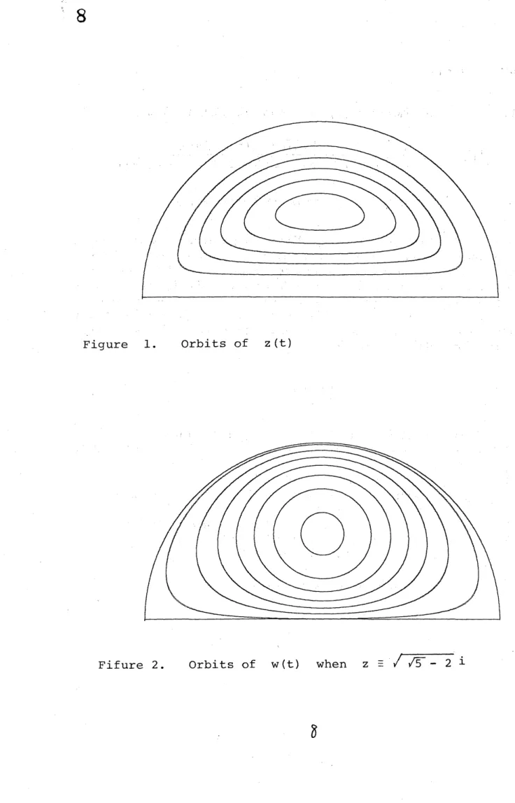
PROPOSITION

1. The system (2.7) is completely integrable and has a unique

$eq$uilibrium:

(2.9) $z=i\sqrt{\sqrt{5}-2}$

Other orbits of (2.7) are periodic ones which surroun$d$ this

$equ$ilibrium, see Figure

1.

PROOF: The essential part of the proof is givenin [2]. We, however, give a complete

proof in our framework. Let us use the polar coordinates (I,$\sigma$) defined by $\sqrt{2I}e^{i\sigma}=$

$z$. Then, by the definition of the Hamiltonian, we have

(2.10) $e^{-4H}= \frac{(1-2I)^{2}8I\sin^{2}\sigma}{4I^{2}+1-4I\cos 2\sigma}$

.

We now introduce some symbols. We put

$A=e^{-4H}$, _$\xi=1-2I$, $f(\xi)=-4\xi^{3}+(4-A)\xi^{2}+4A\xi-4A$. Then (2.10) is rewritten as:

4

Thi$s$ equation defines a family of closed curves in $D_{1}$. If we regard the right hand

side of (2.10) as a function of (I,$\sigma$), then we see that it has one and only

one

maximum at $\sigma=\pi/2,$ $I=(\sqrt{5}-2)/2$. At this point $A$ takes it maximum value

$10\sqrt{5}-22$. If $0<A<10\sqrt{5}-22$, then (2.11) defines a closed curve enclosing

the point (2.9) inside it. On these curves, the motion of $z$ is described as follows.

Taking the real part of (2.5) multiplied by 7, we have

(2.12) $\dot{I}=\frac{1}{2}\cot\sigma-\frac{4I\sin\sigma\cos\sigma}{4I^{2}+1-4I\cos 2\sigma}$

By (2.11,12) we have $\dot{\xi}=(A-\xi^{2})\sqrt{f(\xi)}/(\sqrt{A}\xi^{3})$

.

This equation defines the time

evolution of the vortex $z(t)$ on the closed curves given by (2.11). We can solve this

equstion by means of elliptic functions and see that the solutions are periodic.

_I

By the periodicity of$z$, the equation (2.8) is a system whose Hamiltonian depends

periodically on $t$

.

PROPOSITION 2. The differential equation (2.6) is definable on the $bo$undary

of$D_{1}$

.

The $bo$un$d$ary of$D_{1}$ is invariant with respect to the flow given by (2.6).

$w=1,$ $-1$ are unsta$bleeq$uilibria.

PROOF: The right hand side of (2.6) is equal to the following

(2.13) $\frac{i(\overline{z}-z)(1-|z|^{2})(1-\overline{w}^{2})}{\{\overline{w}^{2}-(z+\overline{z})\overline{w}+|z|^{2}\}\{\overline{w}^{2}|z|^{2}-(z+\overline{z})\overline{w}+1\}}$

It is clear from (2.13) that

$w=-1,$

$+1$ are equilibria. On the boundary

cir-cumference, we have $w=e^{i\gamma}$ _{$(0\leq\gamma\leq\pi)$}

.

In this case, (2.13) is equal to

$c(e^{2i\gamma}-1)=2c\sin\gamma ie^{i\gamma}$, where $c\in R$. This means the vector field is tangent to the

boundary. Similarly it is tangent in the case of $w\in[-1,1]$, since (2.13) $\in R$ when

$w\in R$

.

Therefore the boundary of $D_{1}$ is an invariant set.

:

Thus the equation (2.5,6) has nice properties which (2.3,4) with $\alpha\neq 0$ does not

share. Notice that (2.4) can not be defined on the boundary for $\alpha\neq 0$. Although

(2.5,6) are simpl\‘e, it is connected through $\alpha$ to the equation considered in [1].

Since a similar problem is considered in Aref and Pomphrey $[5,6]$, we would like

to mention our motivation here. In $[5,6]$, they consider the motion of a passive

vortex stirred by three identical vortices. Since this problem is a special case of

three vortices with different intensities, it seems to us that our problem is simpler

5

move

periodically or stationary and there is no motion of other kind. On the other

hand, threevdrtices can move with more varieties, e.g., they can collide ([7]).

Suppose that $z$is the equilibrium (2.9). Then (2.8) is independent of time, which

implies that the Hamiltonian $\tilde{H}$

is constant along individual orbits. Consequently

(2.8) is completely integrable and the orbits of (2.8) consist only of closed Jordan

$t$

curves

defined by $\tilde{H}(w, i\sqrt{\sqrt{5}-2})=$ constant. Furthermore, they occupy the

whole phase space of (2.8) except for the boundary (see Figure 2). If the initial

position of $z$ is placed slightly apart from (2.9), then $z$ moves on a small closed

curve surrounding the equilibrium. In this

case

$\tilde{H}$

is nolonger independent oftime

and complicated orbits may appear. Let $T$ be the period of$z$

.

Then we can obtain

a Poincar\’e map in a usual way:

(2.14) $f:w(0)arrow w(T)$.

We give in APPENDIX a theorem by which the map (2.14) becomes well-defined in $\Omega\equiv\overline{D_{1}}\backslash \{z(0)\}$. This is equivalent to saying that

if $w(O)\neq z(O)$, then $w(t)\neq z(t)$ for all $t$.

If this is proved, it is clear that the map (2.14) is one-to-one, onto and continuous.

Furthermore it preserves the area. Although our “proof” is not complete, we think

the account in APPENDIXis a strong evidence of the correctness of the theorem.

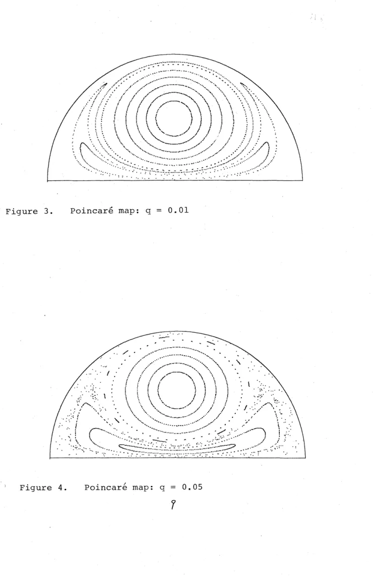
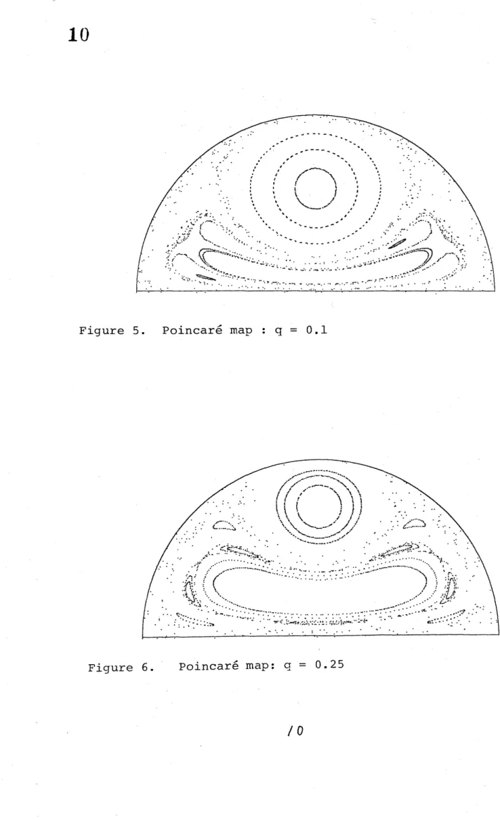
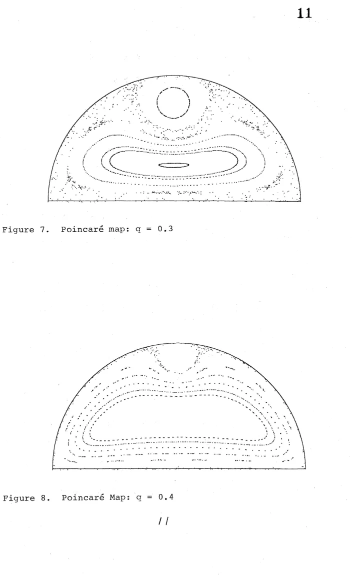
We now examine the properties of the Poincar\’emap. It is enough to consider the

case where $z(0)=iq+i\sqrt{\sqrt{5}-2}$ $(0<q<1-\sqrt{\sqrt{5}-2})$_{. Let the mapping be}

denotedby $f_{q}$ when $z(O)=iq+i\sqrt{\sqrt{5}-2}$ . Severalorbits are drawn on eachfigure$s$ $3- 8$. Figure 3, $\cdots,$ $8$ correspond to $q=0.O1,0.05,0.1,0.25,0.3,0.4$, respectively.

It should be noticed that there is a fixed point in a lower part of the imaginary

axis and that it is enclosed by a layer of closed curves. This shows that there is

a periodic orbit which has exactly the same period as that of $z(t)$ and that it is stable. Some topological argument shows that there must be an unstable fixed

point. Figure 1 shows that the unstable fixed point is on the upper side of the

imaginary axis and that the stable fixed point are connected to the unstable one by a homoclinic orbit. We can observe that the region occupied by the invariant

circles reduces and the islands grows up in accordance with the increase of $q$. We

also notice that, even in the case ofa large $q$, there are KAM tori around the point

$z(O)$. The reason is that, when $w(O)$ is close to $z(O)$, the interaction of $w$ with the

$)$

boundary is negligibly small compared with the interaction between $w$ and $z$ (see

6

Conclusion.

Our equation (2.6), despite its simple appearance, exhibits chaotic

orbits. It seems to the authors that ours is one,of_the simplest equation among the

$chaos-displaying$vortex systems. As is shown in [4], streamlines of a stationary 3-D

Euler flow can be chaotic. Our example shows that 2-D time-periodic Euler flow

may.have chaotic trajectories ofparticles.

APPENDIX

1. Here we prove:

THEOREM A. For any tu$b$ular neighborhood $N$ of _{$O=\{(z(t),t);0\leq t<T\}$},

there is an invariant torus such that it $li$es in $N$ and that $O$ liesinside it

The precise meaning of this theorem is as follows: The phase space of (2.8) is

$\bigcup_{0\leq t\leq T}(\overline{D_{1}}\backslash \{z(t)\})$, where the sections$t=0$ and$t=T$ areidentified. Thereforeit

is homeomorphic to $(\overline{D_{1}}\backslash \{z(0)\})\cross S^{1}$, where $S^{1}$ is a circle. Note that _{$\{z(O)\}\cross S^{1}$}

corresponds to the orbit of$z$. The above theorem asserts that all the neighborhood

of $\{z(0)\}\cross S^{1}$ has an invariant torus which contains $\{z(0)\}\cross S^{1}$ inside.

FORMAL PROOF OF THEOREM $A$: Let us introduce $U+iV=u+iv-z(t)$ where

$u+iv=w$. Then (2.8) is rewritten as

(A.3) $\dot{U}=-\frac{\partial K}{\partial V}$, $\dot{V}=\frac{\partial K}{\partial U}$,

where we have put

$K(U, V,t)= \frac{1}{2}\log\frac{|U+iV||U+iV+z-1/z|}{|U+iV+z-\overline{z}||U+iV+z-1/\overline{z}|}+V{\rm Re}(\dot{z})-U{\rm Im}(\dot{z})$.

Note that the right hand side depends on $t$ through $z=z(t)$. If we define _{$K_{0}(U, V)$}

and $K_{1}(U, V,t)$ by $K_{0}(U, V)= \frac{1}{4}\log(U^{2}+V^{2})$, _{$K_{1}(U, V,t)=K(U, V, t)-$} $K_{0}(U, V)$ then, $K_{1}$ is continuous on $\overline{D_{1}}$, the closure of $D_{1}$

.

Note that the orbits

of $\dot{U}=-\frac{\partial K_{0}}{\partial V}$, $\dot{V}=\frac{\partial K_{0}}{\partial U}$, are simply the circles about the origin. We attempt to

apply the KAM theory to the Hamiltonian system (A.3). Let $\epsilon>0$ be a small

pa-rameter. Weintroduce canonical variables $(p, q)$ by $p= \frac{U^{2}+V^{2}}{2\epsilon^{2}}$, $q=\arg(U+iV)$.

We further change $t$ to $\epsilon^{2}t$. Then (A.3) becomes:

7

where we have put

$(A.5)$ $F=F_{0}(p)+F_{1}(p, q,t, \epsilon)$, with $F_{0}(p, q,t, \epsilon)=\frac{1}{4}\log p$,

$F_{1}(p, q,t, \epsilon)=\frac{1}{2}\log\frac{|\epsilon\sqrt{2p}e^{iq}+z(\tau)-1/z(\tau)|}{|\epsilon\sqrt{2p}e^{iq}+z(\tau)-\overline{z(\tau)}||\epsilon\sqrt{2p}e^{iq}+z(\tau)-1/\overline{z(\tau)}|}$

$+\epsilon\sqrt{2p}\sin q{\rm Re}(\dot{z}(\tau))-\epsilon\sqrt{2p}\cos q1m(\dot{z}(\tau))$,

where $\tau=\epsilon^{2}t$. These are defined on _{$q\in R/2\pi Z$} and _{$p\sim 1$}

.

In this setting we wish

to use Theorem 2 in Arnold [3]. Thi$s$ theorem garantees the existence of invariant

tori for $\epsilon>0$ which is close to unperturbed torus _{$p=p_{0}(\in[1/2,2])$} where $p_{0}$

is sufficiently incommensurable. There is, however, one difficulty that the slowly

changing parameter is $\epsilon t$ in [3], while it is $\epsilon^{2}t$in (A.5). We hope that this diffuiculty

is overcome if we follow the method of [3] indetail. Accordingly we are satisfiedby

the form (A.4) and stop here rather than pursuing rigorous proof, which seems to

require aformidable calculation.

I

REFERENCES

1. Y. Kimura and H. Hasimoto, J. Phys. Soc. Japan 55 (1986),

5-8.

2. Y. Kimura, Y. Kusumoto and H. Hasimoto, J. Phys. Soc. Japan 53 (1984),

2988-2995.

3. V.I. Arnold, Soviet Math. Dokl. 3 (1962), 136-140.

4. V.I. Arnold, “Mathematical Methods ofClassicalMechanics,” Springer Verlag,

New York, Heidelberg, Berlin,

1978.

5. H. Aref and N. Pomphrey, Proc. R. Soc. London A 380 (1982),

359-387.

6. H. Aref and N. Pomphrey, Phys. Lett. A 78 (1980),

297-300.

7.

H. Aref, Ann. Rev. Fluid Mech. 15 (1983), 345-389.

8

Figure 1. Orbits of $z(t)$

$v$

Figure 3. Poincar\’e map: $q=$ 0.01

Figure 4. Poincar\’e map:

$q=0.05$

10

Figure 5. Poincar\’e map :

$q=0.1$

11

Figure 7. Poincar\’e map:

$q=0.3$