スタンダードポテンシャルに束縛されているΨとγの質量準位
12
0
0
全文
(2) Journal of Hokkaido University of Education (Section II A) Vol. 32, No. 1 September, 1981. -ib»iaiicw*¥e% w 2 SB A) us 32« ^ i -f n3W 56 -^ 9 fl. Mass Spectroscopy of 1P and T Bounded in the Standard Potential. Masanobu HIRANO and Tadatoshi KOYANAGI Physics Laboratory, Sapporo College, Hokkaido University of Education, Sapporo 064. IFgf%t • ^m^ij: x ^ >- y- K ^T > ^ + ^^^,^? -fz-C ^ &. ^ b r cosfiws:. »ii'i&ir^!!NL?^mw'»s. Abstract We solve the Schroedinger equation for the quark-antiquark (ec and bb) bounded in the standard potential by the WKB approximation method. We investigate L=0 and L+0 states and determine the model parameters of this system. We compare the results with those of the computer numerical analyses.. § I Introdution The picture of quarkonium levels as nonrelativistic bound states has provided much constructive guidance for experiment, and has made possible many useful inferences from these experiments.. Theoretical efforts may be divided into three categories" ; 1) The adjustment of explicit potentials to reproduce known data and to make predictions for future experiment to confront.. 2 ) The full use of tools of nonrelativistic quatum mechanics. 3 ) To derive the static interquark interaction from QCD. Within the first category in which we have engaged2'"6', three types of the model are proposed at present. Two of them are simple and the other is sophisticated. The first potential71'8' is V(r)=—ag-+^r, r ' '"'. (1-1). which we name the standard potential. The first term is motivated by the asymptotic freedom at a short distance based on QCD. The second term is motivated by the quark confinment at. (17).
(3) Masanobu HIRANO and Tadatoshi KOYANAGI. a large distance which is suggested by the lattice guage theory, the dual string model and the mass level ordering ?-series) which was studied phenomenologically. The second9' is obtained by the gluon exchanges only as,. .2t-_J-J_ _a^A2). V(g-)=-f?. ^33^2N"',^,^q2. l+^l2^ffs(-d2)^. •. (1-2). This is interpolated to the infra-red regions beyond the discontinuity around q2^A2 artificially as ~l/q2 (1+ const. In (l+qz/A2). Of course, the admixture of (1) and (2) have recently been attempted.. The third is given in a more sophisticated fashion as follows,1011". V(r)=-^- r^r,, =log-^- r^r^r^,. =\r. r^r-t,. (1-3). where r, and rz are determined by continuing V(r) and its first derivative. The logarithmic potential at intermediate distances (around 0.5 to 1.5 fm)is a new proposal, where no theoreti-. cal dogma exists. The potential was suggested to explain the T'—T mass splitting identical to the f'—'y mass splitting.12'. We selected the first type of potential due to its simplicity. We have investigated the mass spectroscopy of ec and bb, and ee decay width of these new particles on the basis of the above potential.2>~6) We analysed these by two methods in the pevious papers. The first method is the variation methed introducing the trial harmonic wave function and determining its variable prameter.3' Another one is the WKB quantization method which is useful for the potential including the Coulombic one which is singular at r=0.4> In this article, we report the analyses of the above subject by the WKB approximation method for T in addition to '*$'. We also investigate the eigenvalue of L+0 state. We studied neither of these in the previous paper4'. In § II, we review the WKB method for L=0 states simply along the previous one. In § III, we apply the WKB method to L+0 states and derive the WKB eigenvalue formula. In §IV, we will summarize the results and compare these with those of the computer numerical analyses.. § II L=0 Energy Eigen values in WKB Approach In the previous paper4' we argued in detail the case of L=0 mass spectroscopy by the WKB approximation method.l!i>14> So we will mention the derivation of the WKB eigenvalue formula simply and obtain the improved final results. Based on the theoretical and phenomenological isnvestigation, we consider the standard potential fom the quark-antiquark (ec and bb) system to be. (18).
(4) Mass Spectroscopy of V and T. Ole. V(r)=-^e-+^r.. (2-1). We may write the radial wave equation for the two body system,. ^-^+^^r+M^L-Ewr)-° (2-2) where R(r) is the radial wave function and // is the reduced mass. It is convenient to make a change of variables,. x^,. (2-3). where /=(2/U)-1/3.. Then the radial equation becomes. [-^~(^+x+ L(LX^1) +N)] R(x)=o (2-4) where we use the abbreviation C=2agHl, N^E/e, e-(2^2)-1.. (2-5). Inputting C and L values into eq. (2-4), we obtain the eigenvalues (N). For S states (L=0), the WKB eigenvalue condition is. j /goUcV dx= (n+^)jr (2-6) with g,(x)=N-x+^-,. (2-7). while Xi the classical turning point (N—XI+C/XI=O) may be applied to negative ones as well as to positive eigen values.. Secondly, substituting a new variable u by putting x=v2(l-u2),. (2-8). where v2=( N2+W+N)/2 is one of the solution of Nx-x2+C=0, we can do eq. (2-6) with tedious calculation and obtain. {^' ^xTdx=^A[A-^NF(ks)+M E(k2)] (2-9) where. A==/7V2+4C .,_. VN2+W+N. 2/]V2+4C. (19). (2-10).
(5) Masanobu HIRANO and Tadatoshi KOYANAGI 1. •[. w)=^ Al-u^-k-^ du' ^=!^1Y^/ ~ d-' (2-11) and F(k2)(E(k2)) is the complete elliptic integral of the first (second) kind."' Then we obtain the final expression of the WKB eigenvalue formula for S-states,. /A[AjNF(k2)+m- E(k2)^ =(w+|-) TT, (2-12) which is deformed as A3=. 9(%+-1)2^2. T. Wl-k2)F(k2)+(2k2-l)E(k2)] <2-13). From this, we determin the value of A for the arbitrary set of n and k, and also the values of N and C, using N'=A(2kt-l) and C=(Al-N2)/'i of eq.(2-10). § III L^:0 Energy Eigenvalues in WKB Approach For L+0 states, the WKB eigenvalue condition for eq. (2-4) is. Gi=fxz^xVdx=(n+^)n, (3-1) gi(x)=N-x+c^-c^, X X'. (3-2). where Xi<Jk, the two classical turning points ( gi(xi)=0, gi(xs)=0 ) which may be applied to negative ones as well as to positive eigenvalues (N) and d., is (case I) CL=:L(L+I), (case II) Ci.=(L+l/2)2. The above replacement of (L+1/2) 2 in the centrifugal term instead of L(L+1) is based upon the problem of the attractive Coulomb field.14' This is essential to obtain the well-known eigenvalue relation with the principal quantum number. We will investigate both cases in the following WKB approximation method. The integral (3—1) may be evaluated in four steps. First substituting a new variable by putting y2=a-x,. (3-4). where a is one of the real solution for gi{x)=0 and we may take a=Xt. Eq. (3—1) is written as "^ 2v^.i/f+(N-3a).i/2+(3a2-2aN-C)] ^, Tl~-]»t (y2-a)^+^N=3a)y2+(3a2-2aN:=~C) ""'. (20).
(6) Mass Spectroscopy of f and T. and r- 2^2-/.2)(^-.2). G(=^ {y^^y^W^1} dy' (3-5) where yi= V a—Xi y2=^a-X2=0,. v2=[(3a-N)+^-3ci2+2aN+N2+4C ]/2, v2=[(3a-N)-^-3a2+2aN+N2+4C ]/2. ^_^ This may be followed by a second substitution of y2=ti2. ti2. (3-7). which leads to a integral with k2=/^2/v2 •^__2^ni(u'-l)(^u'-v'. G'^o7(^7^)7(^T<2)a-A2.2T ^ (3-8) In the third, we rearrange eq. (3-8) as follows,. Gi=l-[-^L+^(^+v2-a)h-(fz2-a)(^-a)Io+(^-a)(v2-a)U(ks)], (3-9) where •i. u'. ^ Al-u2)(l-k2u2) {> 1. ,. (3-10). /7(^2)= /„ —„. , ^_,,- du, /° (i—^u2)^U~-ua)(l-k2u2). and II (kz) is the complete elliptic integral of the third kind. Using the recurrence formula of 115> and the relation18'. Q(k2)=F(k2)+^^\.l-Ao(k2//3)], (3-11) where Ao is Heuman's lambda function and /3=sin-lW-t2)/cos2a], ^=Wl-t2)-l(t2-sinaa)]w,. (3-12). t2=^/a, then we obtain the final expression of the integral (3—1), Gi=F(t2,k2)a/a~. (3-13). where. F(t\ks)=^-^k—[(2k2tz+t2-3k2)F(k2)+(-k2t2-t2+3k2)E(k2)] (21).
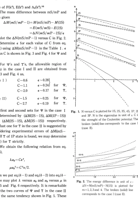
(7) Masanobu HIRANO and Tadatoshi KOYANAGI. (l-t2)(t2-k2. p. +7T. (3-14). [A»(k2//3)-l].. Therefore the WKB eigenvalue formula for L^O is given as. F{t\k2)a/a~=(n+^))t.. (3-15). We may also express N, C and CL by means of t2,k2 and a :. N=(3-t2-^a, ft /•!. (3-16). C=(-3+2(2+^-^a2, C^=(-l+t2+. t2. t4. ^3.. Taking arbitrary sets of n, k2 and t2, we get the value of a from eq. (3-15) through the table F(k2), E(k2) and Ao(k2//?).18> We determine N, C and CL values from eq. (3-16). As CL is restricted to the case I and case II, we may select the specific sets of k2 and t2. By means of this procedure, we obtain the relation of N versus C.. We note that case I with L=0 tends to the result in § II exactly, but case II with L=0 gives a different result. It is important to compare both cases for L=0 states bounded in the standard potential (eq. (2—1)) as well as for the Coulomb potential only"'. § IV Result and Discussion Our purpose is to interpret 'V and T mass spectroscopies by the standard potential. In other. words, nobody knows the exact type of the potential, so that it is important to determine the potential adjustable to the experimental masses of Vs and T's. We note that we will investigate both case I and II of the replacement in the centrifugal potential term in the following. Our input data are given in the table I. Table 1. Experimental values of mass and mass difference for ip and T ""• 17). M (IS) M (2S) M(3S) M (4S). 9. T. 3097 ± 2 (MeV). 9434.5±0.4. 3686 ± 3. 9993.0±1.(). 4040 or 4028. 10323.2±0.7. 4415±10. 10570.0. M (2S-1S). 589 ± 4 (Me V). 559.0±0.2. M (3S-1S). 940 ±50. 889.0±I.O±4.0. M (4S-1S). 1318±10. 1114.0±2.0±5.0. M (1P-1S). 426±4. (MeV). (MeV). First, we show the relation of N versus C for L=0 states ( lS(n=0), 2S(n=l), 3S(n=2) and 4S(n=3) and L=l states (lP(n=0), 2P(n=l) and 3P(n=l) and 3P(n=2) is Fig. 1. We used the. (22).
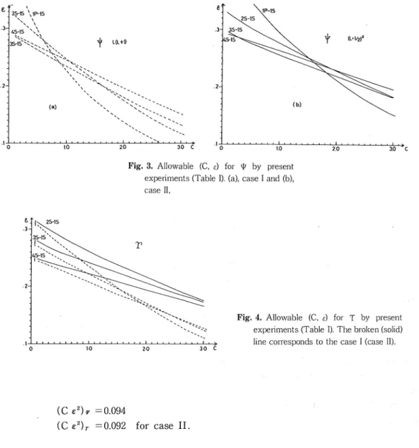
(8) Mass Spectroscopy of V and T. table of F(k2), E(k2) and Ao(k2).18' The mass difference between mS/mP and IS is giuen. ^M(mS/mP-l}=M(mS/mP)- M(1S) =E(mS/mS)-E(lS) =^N(mS/mP-lS)/e We plot the AN(mS/mP-l) versus C in Fig. 2. We determine e for each value of C from eq.. (4-1) using AM(mS/mP-l) in the Table I. e versus C is shown in Fig. 3 and Fig. 4 for 'P and r.. For T's and T's, the allowable region of (C, e) in the case I and II are obtained from Fig. 3 and Fig. 4 as, .case. I). (case II). C-0.6. e~0.28|. C-l.l. e~0.24j. for. 1P,. C-2.0. e~0.17. for. T,. C-1.5. e-0.25. for. ^,. C-2.7. e-0.19. for. r.. The first and second sets for ^ in the case I. are determined by (AM(2S-1S), AM(IP-IS)). Fig. 1. N versus C is plotted for IS, 2S, 3S,4S, IP,2P and 3P. N is the eigenvalue in unit of e. C is. the strenght of the Coulombic potential. The. and (AM(2S-1S), AM(3S-1S)) respectively.. broken (solid) line corresponds to the case I. The last one for T in the case II is suggested by considering experimental errors of AM(mS—. IS). If T of IP state is found, we may determine. (case II). AN 10-1. (C, e) for T strictly. We obtain the following relation from eq. (2-5), 5-| \ag=Ce2,. fza/=C2e/2. When we put eq.(4—l) and eq.(4—2) into eq.(4—. 0. 1.0. 2.0. ''''''. 30'i. 3), we may plot A. versus ag and ag versus p. in. Fig. 2. The energy difference in unit of e :. Fig. 5 and Fig. 6 respectively. It is remarkable. AN=N(mS/mP)-N(lS) is plotted for. that the two curves of f and T in the case II. m=l,2,3and 4. The broken (solid) line. take the same tendency shown in Fig. 5. These. corresponds to the case I (case II).. features are also suggested in the case I in Fig. 5. This indicates Ce2~ constant common to '9 and T.. The values of them are. (23).
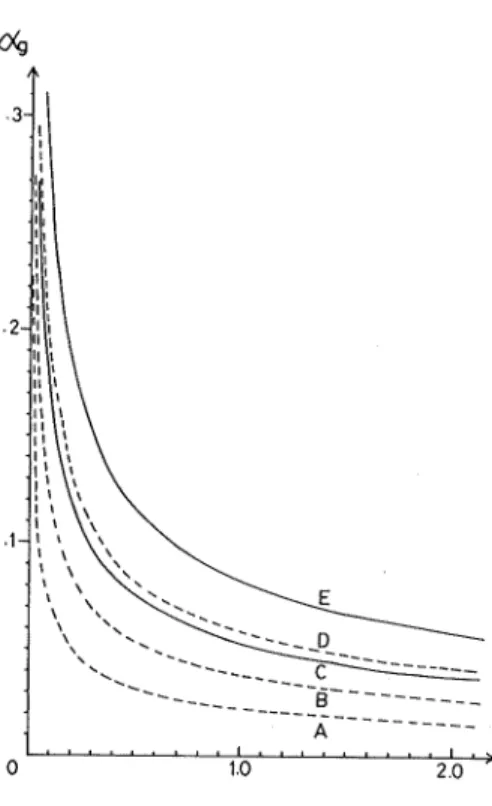
(9) Masanobu HIRANQ and Tadatoshi KOYANAGI. 2S-S \IP-1S. \\. t15 "Y\ !3S-1S'^;,.\,. <:^ "\~;'. ^ (L.l/2)'. <|) L(L+. "^Y (a). Fig. 3. Allowable (C, e) for >P by present. experiments (Table I), (a), case I and (b), case II,. (^25-IS. Fig. 4. Allowable (C, e) for T by present experiments (Table I). The broken (solid) 30 C. line corresponds to the case I (case II).. (Ce2)y =0.094. (C. =0.092 for case II.. In the previous paper, we compared our results with DESY and CORNELL parameters,8"" (DESY) fi=O.SQGeV A.=0.171Gev2 ffg=0.55,. (CORNELL) f^=0.92GeV A=0.183GeV2 ^=0.52. Comparing those with our improved results, we find the following set of parameters for the case 11 from Fig. 5 and Fig. 6, fz=O.SOGeV Ji=0.153GeV2 ag=0.593, /<=0.92G<,y Ji=0.169GeV2 ^=0.552.. which mostly resemble DESY and CORNELL respectively. In the last, we show the computer analyses (numerical computation of eq. (2—2)).61. (24).
(10) Mass Spectroscopy of f and T. \. ^. !l.'. ;;. I. .6-. .3-1. I^ !i. .5-. l;l ! 'i i II. ',". In. I II. ^\\\. .4-. •2-{. '. 1\. ^. \\'. .3-. *, v<. \ *.\. '' 'N. > '.\. v^'.. .2-. •l-l. \ \\. \ '••\. \'^'. .-. ^t <\'.. ?6. \ '. .1. ^<^c;. A ~~--^ -I—> 1.0 0(g. .5. 2.0. 1.0. Fig. 5. The relation of A versus a, for >p and T. The. Fig. 6. The relation of ag versus /; for f and T. Par-. broken (solid) line corresponds to the case I. ameters are the same as ones in Fig. 5.. (case II). Parameters are given by A (C= 0.6, £=0.28GeV), B (C=l.l, e=0.24GeV), C (C=1.5, e=0.25GeV), D (C=2.0, e=0.17 GeV) and E (C=2.7, £=0.19).. £/ .4-1. 25-15 .3-1 •3-1. .2-1. 45-15. .2-1. 0. 1.0. 0. 'C. Fig. 7. Allowable (C, , 1 for y8' by present experiments. (Table 1). AM(3S-1S),. 1.0. 2.0. 3.0. ~"c. Fig. 8. Allowable (C, s) for T by present experiments. -for AM (2S-1S), ——-for. (Table 1).. -foi-AM(2S-lS),- —-for AM. -for AM(4S-lS)and—.-. (3S-1S). --—for AM(4S-1S). Each allowable. for AM(IP-IS). CORNELL and DESY are. region crosses nearly at (C, s)~ (2.65, 0.18. given in the paper.. GeV).. (25).
(11) Masanobu HIRANO and Tadatoshi KOYANAGI. Allowable (C, e) for "c? and T are given in Fig. 7 and Fig. 8. Input data are the same as in Table 1. The allowable (C, e) regions which are determined from the Fig's have narrow common region,. (C,e)y-(1.347, 0.2634 GeV) for DESY, (1.375, 0.2630 GeV) for CORNALL, (C,e)r~(2.65, 0.18 GeV), and Ce2=0.093 or 0.095 for ^, Ce2=0.086 for T. These are consistent with the result of the case II.. In this paper, we try to solve eq. (2—2) using the WKB approximation method. Because the standard potential includes the singular one (ag/r) at r=0, we replace (L+ 1/2 )2(case II) instead of L(L+l)'(cffse I) in the centrifugal potential term according to the treatment of the Coulomb field.14' This indicates that the above replacement is important for the standard potential in the WKB approach. This methed gives useful information of energy eigenvalues and model parameters for "9 and T. The noteworthy point is that V and T have the common values for Ce2. In the near future we will examine closely other work,19' which has been done recently with the same view point as ours. A comparison of these will provide more understanding of the structure of quarkantiquark system.. Referneces. 1) C. Quigg and J. L. Rosner, Prep. FERMILAB-PUB-79/22-THY. C. Quigg, Prep. FERMILAB-Conf-79/74-THY. 2 ) M. Hirano and Y. Matsuda, Prog. Theo. Phys. 60(1978), 1490 ; Prog. Theo.. Pbys. 62(1979), 501. 3 ) M. Hirano and Y. ikeda, Jounal of Hokkaido Univ. of Education, Sect. 11 A 30(1979), 19. 4 ) M. Hirano and H. Yamaguchi, Jounal of Hokkaido Univ. of Education, Sect. II A 31(1980), 15. 5 ) Y. Abe, K. Fujii, M. Hirano, Y. Hoshino, K, Honda, K. Iwata and T. Murota, Frog, Theo. Phys. 60(1978), 639. Y. Abe, K. Fujii, M. Hirano, Y. Hoshino, K. Iwata and T. Murota, Frog. Theo. Phys. 61(1979), 1566. Y. Abe, K. Pujii, M. Hirano, K. Honda, Y. Hoshino, K. Iwata, T. Murota and T. Okazaki, Prog. Theo.. Phys. 63(1980), 1078. 6 ) M. Hirano, K. Iwata, K. Kato and T. Murota, Prog. Theo. Phys. 65(1981), 983. 7 ) T. Appelquist, R. M. Barnet and K. D. Lane, Prep, SLAC-PUB-2100, 1979. 8 ) E. Eichiten, K. Gottfried, T. Kinoshita, K. D. Lane and T. M. Yan, Phys. Rev. D21(1980), 203. 9 ) W. Celmaster and F. S. Heney, Phys. Rev. D18(1978), 1688. R. Levine and Y. Tomozawa, Phys. Rev. D19(1979), 1572.. J. L. Richardson, Phys. Letters 82B(1979), 272. D. Ito, Prep. SUPITSOOl-Saitama Univ., 1980. 10) M. Krammer and H. Kraseman, "Qnarkonia", Lectures presented at Infernationale Uniuersitatswochen filr. Kernphysik, Austria 1979.. (26).
(12) Mass Spectroscopy of 9 and T 11) G. Bhanot and S. Rudaz, Prep. DESY-79-09, 1979. J. S. Kang, Prep. RU-79—148 Rutgers Univ., 1979.. 12) C. Quigg and J. L. Rosner, Phys. Letters 71B(1977), 153. 13) M. Alonso and H. Valk, Quantum Mechanics, (Addison-Wesley, 1973) p. 181. 14) S. FlUgge, Practical Quantum Mechanics (Springer-Verlag, 1974) p. 303.. 15) ^a^-, ^EBJUI^, -^{8 ;®:^fi^(I) (S%, 1973) P.140.. 16) Partical Data Group, Rev. Rod. Phys. 52 No.2(1980). 17) D. Andrews etal., Phys. Rev. Letters 44(1980), 1108.. T. Bohlinger et al, Phys. Rev. Letters 44(1980), 1111. is) i?- ^a^-; (m, 1976) P.318. M. Abramowitz and I. A. Stegan, Handbook of Mathematical Functions (Douer, 1972) p 587. 19) M. Kaburagi, M. Kawaguchi, T. Morii, T. Kitazoe, and J. Morishita, Phys. Letters 97B(1980), 143. N. Barik and S. N. Jena, Phys. Rev. D21(1980), 2647 ; Phys. Rev. D21(1980), 3197 ; Phys. Rev. D22(1980), 1704 ; Phys. Letters 97B(1980), 265. H. Suura, W. J. Wilson and Bing-lin Young, Phys. Rev. D21(1980), 3204. W. Buchmuller, G. Grunberg and S. H. H. Tye, Phys. Rev. Letters, 45(1980), 103.. (27).
(13)
図

関連したドキュメント
Recently, Velin [44, 45], employing the fibering method, proved the existence of multiple positive solutions for a class of (p, q)-gradient elliptic systems including systems
Related to this, we examine the modular theory for positive projections from a von Neumann algebra onto a Jordan image of another von Neumann alge- bra, and use such projections
In Section 13, we discuss flagged Schur polynomials, vexillary and dominant permutations, and give a simple formula for the polynomials D w , for 312-avoiding permutations.. In
Analogs of this theorem were proved by Roitberg for nonregular elliptic boundary- value problems and for general elliptic systems of differential equations, the mod- ified scale of
“rough” kernels. For further details, we refer the reader to [21]. Here we note one particular application.. Here we consider two important results: the multiplier theorems
“Breuil-M´ezard conjecture and modularity lifting for potentially semistable deformations after
In my earlier paper [H07] and in my talk at the workshop on “Arithmetic Algebraic Geometry” at RIMS in September 2006, we made explicit a conjec- tural formula of the L -invariant
Then it follows immediately from a suitable version of “Hensel’s Lemma” [cf., e.g., the argument of [4], Lemma 2.1] that S may be obtained, as the notation suggests, as the m A
