JAIST Repository: 相関ルールマイニングにおける冗長性削減アルゴリズムに関する研究

全文

(1)JAIST Repository https://dspace.jaist.ac.jp/. Title. 相関ルールマイニングにおける冗長性削減アルゴリズムに関する研究. Author(s). 鈴木俊行. Citation Issue Date. 2002-03. Type. Thesis or Dissertation. Text version. author. URL. http://hdl.handle.net/10119/375. Rights Description. Supervisor:Ho Tou Bao, 知識科学研究科, 修士. Japan Advanced Institute of Science and Technology.

(2) 修. 士. 論. 文. Reducing the redundancy in association rule by frequent closed itemsets. 指導教官. Ho Tou Bao. 教授. Japan Advanced institute of science and technology Knowledge Science Knowledge system science. 050045 Toshiyuki Suzuki. 審査委員：. Ho Tou Bao 教授（主査）石崎. 雅人教授. 中森. 義輝教授. 佐藤. 賢二教授. 2002 年２月 Copyright Ⓒ 2001 by Toshiyuki Suzuki. i.

(3) Content Chapter 1 Introduction. 1 1.1 Data mining and Association rules . . . . . . . . . . . . . . . . . . 2 1.2 Research objectives . . . . . . . . . . . . . . . . . . . . . . . . . . . . . . .3 1.3 Contribution of the work . . . . . . . . . . . . . . . . . . . . . . . . . . 4 1.4 Organization of the thesis . . . . . . . . . . . . . . . . . . . . . . . . . 4. Chapter 2 Association rule mining. 5 2.1 A framework of association rule mining . . . . . . . . . . . . . . .6 2.1.1 find frequency items in data mining context . . . . 6 2.1.2 Generate the rules based on frequency items . . . .7 2.2 Apriori algorithm . . . . . . . . . . . . . . . . . . . . . . . . . . . . . . . . . 8 2.2.1 Join step in Apriori algorithm . . . . . . . . . . . . . . . .10 2.2.2 Prune step in Apriori algorithm . . . . . . . . . . . . . . 11 2.2.3 Algorithm of Apriori . . . . . . . . . . . . . . . . . . . . . . . .12 2.3 Problems of redundant rules in association rule . . . . . . . .15. Chapter 3 Frequent closed itemsets. 16 3.1 Discover frequent closed itemsets . . . . . . . . . . . . . . . . . . . 16 3.1.1 Frequent closed itemsets thesis . . . . . . . . . . . . . .16. 3.1.2 Algorithm Deriving Frequent Closed Itemsets from frequent itemsets . . . . . . . . . . . . . . . . . . . . . . . . . . . . . . . . . . . . . . . . .17 3.2 Generate generators based on frequent closed itemsets . .21 3.3 Frequent itemsets vs. frequent closed itemsets . . . . . . . . .23. Chapter 4 Strong non-redundant association rule. 25 4.1 Lakhal’s definition vs. Strong definition . . . . . . . . . . . . . .25 4.2 Rules with confidence 100% . . . . . . . . . . . . . . . . . . . . . . . .27. ii.

(4) 4.3 Confidence with lowers than 100% rules . . . . . . . . . . . . . .31. Chapter 5 Efficient algorithm based on Zaki’s algorithm 39 5.1 minimal antecedent and minimam consequent rules . . . .39 5.2 Rules with confidence 100% rules . . . . . . . . . . . . . . . . . . . 41 5.3 Confidence with lowers than 100% rules . . . . . . . . . . . . . .43. Chapter 6 Experiments. 45 6.1 Experimental designs. . . . . . . . . . . . . . . . . . . . . . . . . . . . . .45 6.2 Experimental results. . . . . . . . . . . . . . . . . . . . . . . . . . . . . . 46 6.2.1 Apriori vs. Lakhal’s algorithm. . . . . . . . . . . . . . . .46 6.2.2 Lakhal’s algorithm vs. Strong algorithm. . . . . . . 47. Chapter 7 Conclusion. 48. References…………………………………………………………50. iii.

(5) List of figures ２．１. Lattice structure ．. ２．２. Extracting frequent itemset from D by Apriori algorithm ．. ．. ．. ．. ．. ．. ．. ．. ．. ３．１ Deriving frequent closed itemsets from frequent itemsets. ．. ．. ．. 8. ． 14. ．. ．．． 20. ３．２ frequent itemsets vs. frequent closed itemsets on the lattice structure ．．．．．．．．．．．．．．．． 24 ４．１. generate rules on the lattice ．．．．．．．．．． 30. ４．２. Rules based on Lakhal’s definition ．．．．．．. ４．３. Lakhal definition vs. strong definition ．. ４．４. generate rules confidence with lower than 100% ．. ４．５. Lakhal definition vs. strong definition ．. ５．１. frequent closed itemset lattice ．．．．．．．．． 40. ５．２. Rule based original theorem ．．．．．．. ５．３. Rule based generator. ５．４. Rule based original theorem ．．．．．．. ５．５. Rule based generator. ６．１. Apriori vs. Lakhal algorithm ．. ６．２. Lakhal algorithm vs. strong algorithm ．．．．．．． 47. ．．. ．．. ．．．．．．. ．．．. 30. ．．．．．. ．．．. ．. 31. ．37 ．. 38. ．．． 41. ．．．．．42 ．．． 43. ．．．．．．．．．．． 44. iv. ．. ．. ．. ．. ．. ．. ．. ．46.

(6) List of Tables ２．１. Data mining context ．. ．. ．. ．. ．. ．. ．. ３．１. frequent itemsets vs. frequent closed itemsets. ．. ．. ．. ．. ． 24. ４．１. generated rules confidence with lower than 100%. ６．１. datasets. ．. ．. ．. ．. ．. ．. ．. ．. v. ．. ．. ．. ．. ．. ．．. ．. ．．. ．．. ．. 6 37. ． 45.

(7) Chapter 1. Introduction 1.1 Data mining and association rule mining Knowledge Discovery in Database (KDD) the rapidly growing interdisciplinary field that merges together database, statistics and machine learning-aims to extract useful and understandable knowledge from large volumes of data. Data mining is the main step of the KDD process that performs the extraction of unknown knowledge in data. Association rule mining finds interesting associations and correlation relationships among a large set of items. With massive amounts of data continuously being collected and stored, many industries are becoming interested in mining association rules from their databases. The discovery of interesting association relationships among huge amounts of business transaction records can help in many business decision making process, such as catalog design, cross-marketing, and loss-leader analysis. A typical example of association rule mining is market basket analysis. This process analyzes customer-buying habits by finding associations between the different items that customer place in their “shopping baskets”. The discovery of such association can helps retailers develop marketing strategies by gaining insight into which items are frequency purchased together by customers. The purpose of association rule extraction, introduced [1], is to discover significant relations between binary attributes extracted from databases. An example of association rules extracted from a database of supermarket sales is: “cereal ∧ sugar → milk (support 7%, confidence 50%)”. This rule states that the customer who buy cereals and sugar also tend to buy milk.. 1.

(8) The support defines the range of the rule, i.e. the proportion of customers who bought the three items among all customers, and the confidence defines the precision of the rule, i.e. the proportion of customers who bought milk among those who bought cereals and sugar. An association rule is considered relevant for decision making if it has support and confidence at least equal to some minimal support and minimal confidence thresholds, min_support and min_confidence, defined by user.. 1.2 Research objectives Association rule mining produced many rules. Therefore we have two problems: First: the cost of calculation to find association rules is high. Second: evaluate of association rules is difficult. Many researchers consider some kinds of solutions to above problems. We divide three categories of these researches. Category 1: Efficient algorithm for mining frequent itemsets [5]. This category’s research objects to enumerate all frequent itemsets. Category 2: Mining interesting association rules [2]. This category’s research objects to incorporates user-specified constrains on the kind of rules generated or to define objects metrics of interesting. Category 3: Non-redundant association rules by Zaki [7], Lakhal [4]. This category’s research objects to generate non-redundant association rules. We focus on non-redundant association rules, because association rules are evaluated by users, if we have many rules; The cost of evaluating them will be very high. So we try to reduce the non-informative association rules, by generating only non-redundant association rules.. 2.

(9) We have three objectives in trying to reduce the non-informative association rules. 1. To investigate the problem of non-redundant association rules. 2. To try to formulate another form of non-redundant association rules. 3. To develop an algorithm that finds non-redundant association rules. 4. To try to improve the algorithm.. 1.3 Contribution of the work In the rest of paper, two kind of association rules are distinguished: 100% confidence rules under 100% confidence rules. The solution proposed in this paper consists of generating bases, or reduced covers for association rules. These bases contain non-redundant rules, being thus of smaller size. Our goal is to limit the extraction to the most informative association rules from the point of view of the user with respect to strong association rules. Using the semantic for the extraction of association rules based on the closure of the Galois connection [10], the generic bases for 100% confidence association rules and the informative basis for under 100% confidence association rules are defined. Rules are constructed using the frequent closed itemsets and their generators, and they minimize the number of association rules generated while maximizing the quality of the information conveyed. They allow us to do 1. The generation of only the most informative non-redundant association rules, i.e. of the most useful and relevant rules: those having a minimal antecedent and maximal consequent. Thus redundant rules, which represent in certain databases the majority of extracted rules, particularly in the case of deuce or correlated data for which the total number of valid rules is very large, will be pruned.. 3.

(10) 2. The presentation to the user of a set of rules conveying all the attributes of the databases, i.e. containing rules where the union of the antecedents is equal to the unions of the antecedents of all the association rules valid in the context. This is necessary in order to discover rules that are “surprising” to the user, which constitute important information that it is necessary to consider [11, 12, 13]. 3. The extraction of a set of rules without any loss of information, i.e. conveying all the information conveyed by the set of all valid association rules. It is possible to deduce efficiently, without access to the datasets, all valid association rules with their supports and confidence from databases. The union of these two bases thus constitutes a small non-redundant generating set for all valid association rules, their supports and confidences.. 1.4 Organization In section 2, we recall the basic notions in association rule mining. In section 3, we present frequent closed itemsets that is key concept of our research. In section 4, we try to develop a new definition on non-redundant association rules. In section 5 we improve the algorithm given Zaki. Chapter 6 we present datasets and our experiments for evaluation, and section 7 concludes this paper.. 4.

(11) Chapter 2. Association rule mining In this chapter we present a framework of association rule mining and the most popular and traditional algorithm “apriori”.. 2.1 A framework of association rule mining The association rule extraction is performed from a data-mining context. This framework of association rule mining has two steps, to find frequency items, to generate rules based on frequency items.. Definition 1 (Data mining context) A data-mining context is defined as D = (T , I , δ ) , where T and I are finite sets of transactions and items, respectively, and δ ⊆ T × I is a binary relation. Each couple (t, i ) ∈ δ denotes the fact that transaction t ∈ T is related to the item i∈I .. 5.

(12) Example 1. A data-mining context D constructed of six transactions (each one identified by its TID ) and five items is represented in the fig. 1. This context is used as support for the example in the rest of the paper.. TID 1 2 3 4 5 6. Item ACTW CDW ACTW ACDW ACDTW CDT. Table 2.1. Data mining context D. 2.1.1 Find frequency items in data-mining context In this part, we present how to discover the frequency items in data mining context. Definition 2 (Galois connection) Let D = (T , I , δ ) be a data-mining context, 2 T the set of subsets of T, 2 I the set of subsets of I, and. φ : 2 T → 2 I , φ (O) = {i ∈ I | ∀t ∈ T , (t , i ) ∈ δ }, O ⊆ T φ associates with O items common to all transactions t ∈ T ϕ : 2 I → 2T ,ϕ ( A) = {t ∈ T | ∀i ∈ I , (t , i ) ∈ δ }, A ⊆ I. ϕ associates with an itemset A the transactions related to all items i ∈ l The couple of applications (φ , ϕ ) is a Galois connection between the power set of T. ( 2 T ) and power set of I ( 2 I ). The following properties hold for all I , I1 , I 2 ⊆ I and T , T1 , T2 ⊆ T :. 6.

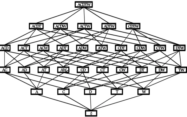
(13) (1) I 1 ⊆ I 2 ⇒ ϕ ( I 1 ) ⊆ ϕ ( I 2 ) (2) T1 ⊆ T2 ⇒ φ (T1 ) ⊆ φ (T2 ) (3) T ⊆ ϕ ( I ) ⇔ I ⊆ φ (T ) Definition 3 (frequent itemsets) A set of items l ⊆ I is called an itemset. The support of an itemset l is the percentage of transactions in D containing l : Support (l ) = | ϕ (l ) | / | O | l is a frequent itemset if support (l ) ≥ min_support.. Lattice structure The set of all itemsets has the lattice structure. It is easy to represent the itemsets to use lattice. A lattice Lk has two features: 1. There exist a partial order on the lattice elements. 2. All subsets of Lk have one greatest lower bound, the join element and one lowest upper bound, the meet element. Given | I | = m, there are possibly 2 m frequent itemsets, which form a lattice of subsets over I with height equal to m. Consider this example, m = 5, we can calculate the possibly 32 itemsets and the lattice with height 5 as shown in Figure 1.. 7.

(14) ACDTW. ACDT. ACDW. ACTW. ADTW. CDTW. ACD. ACT. ACW. ADT. ADW. ATW. CDT. CDW. CTW. DTW. AC. AD. AT. AW. CD. CT. CW. DT. DW. TW. A. C. T. D. W. ０. Figure 2.1. Lattice structure. 2.1.2 Generate the rules based on frequency items In this part, we present how to generate the rules based on frequency itemsets. Once the frequent itemsets from transaction database D have been found, it is straightforward to generate strong association rules from them. This can be done using the following equation for confidence, where the conditional probably is expressed in terms of itemset support count; Confidence(I1 → I 2 − I1 ) = P( I 2 − I 1 | I 1 ) =. sup_ count (I 2 − I 1 ∪ I 1 ) sup_count(I 1 ). Where sup_ count (I 2 − I 1 ∪ I 1 ) is the number of transaction containing the itemsets (I 2 − I 1 ∪ I 1 ) and sup_count(I1 ) is the number of transaction containing the itemsets (I1 ) . Based on this equation, association rules can be generated as follows.. 8.

(15) -For each frequent itemsets l , generated nonempty subsets of l . -For every nonempty subsets of l , out put the rule “ l1 → (l 2 \ l1 ) ” if this rule’s confidence satisfy the minimum confidence, minimum confidence is a threshold defined by user.. Definition 5 (association rules) An association rule r is an implication between two frequent itemsets l1 , l 2 ⊆ I of the form l1 → (l 2 \ l1 ) where l1 ⊂ l 2 . The support and the confidence of r are defined as: support (r ) =support (l 2 ) and confidence (r ) = support (l 2 ) /support (l1 ) . If association rules satisfy the min_support and min_confidence, then we called theses association rules “Strong”.. Example2 These examples are association rules based on Fig1 dataset. We called itemsets on the left side “antecedent”, right side “consequent”. 1) A → CW ( support = 4, confidence = 100% 2) D → C ( support = 4, confidence = 100% ) 3) C → W ( support = 5, confidence = 75.0% ) 4) AW → T ( support = 3, confidence = 83.3% ) These rules means if we find antecedent, we can find consequent on confidence percentage, and these rules occur support count in the analyzing database.. 9.

(16) 2.2 Apriori Algorithm Apriori is an influential algorithm for mining frequent itemsets for Boolean association rules. The name of the algorithm is based on the fact that algorithm uses priori knowledge of frequent itemset property. Apriori employs an iterative approach known as a level-wise search, where k-itemsets are used to explore (k+1)-itemsets. First, the set of frequent 1-itemsets is found. This set is denoted L1 . L1 is used to find L2 , the set of frequent 2-itemsets, which is used to find L3 ,. and so on, until no more frequent itemsets can be found. The finding of each Lk requires one full scan of the database. The Apriori algorithm has two steps. 1st is join step and 2nd is prune step.. 2.2.1 Join step in Apriori algorithm To find Lk a set C k of candidates k-itemsets is generating by joining Lk −1 with itself. This set of candidates is denoted C k . Let l1 and l 2 be itemsets in Lk −1 . The notation l i [ j ] refer to the j th item in l i . By convention, Apriori assumes that items within a transaction or itemset are sorted in lexicographic order. The join Lk −1 >< Lk −1 , is performed, where members of Lk −1 are joinable if their first (k-2) items are in common. That. is,. members. l1. and. l2. of. Lk −1. are. joined. The if (l1 [1] = l 2 [1]) ∧ (l1 [2] = l 2 [2]) ∧ ... ∧ (l1 [k − 2] = l 2 [k − 2]) ∧ (l1 [k − 1] < l 2 [k − 1]) . condition l1 [k − 1] < l 2 [k − 1] simply ensure that no duplicates are generated. The resulting itemset formed by joining l1 and l 2 is l1 [1]l1 [2]...l1 [k − 1]l 2 [k − 1] .. 10.

(17) 2.2.2 Prune step in Apriori algorithm C k is superset of Lk , that is, its member may or may not be frequent, but all frequent k-itemsets are include in C k . A scan of the database to determine the count of each candidate in C k would result in the determination of Lk . C k , however, can be huge, and so this could involve heavy computation. To reduce the size of C k , the Apriori property is used as follows. Any (k-1)-itemset that is not frequent cannot be a subset of a frequent k-itemset. Hence, if any(k-1)-subset of a candidate k-itemset is not in Lk −1 , then the candidate cannot be frequent either and so can be removed from C k . This subset testing can be done quickly by maintaining a hash tree of all frequent itemsets.. 11.

(18) 2.2.3 Algorithm of Apriori Apriori algorithm Input: Database D of transactions, minimum support threshold min_sup Output: L, frequent itemsets in D 1.L1 = find_frequent_1-itemsets(D); 2.for (k=2; Lk-1¹ Æ; k++) { 3. Ck = apriori_gen(Lk-1, min_sup) ; 4. 5. 6.. for each transaction t Î D { /* scan D for count */ Ct = subset(Ck,t) ; /* get subsets of t that are candidate */ for each candidate c Î Ct. 7. 8.. c.count++ ; } Lk = {c Î Ck | c.count ³ min_sup}. 9.} 10.return L = Èk LkProcedure apriori_gen(Lk-1: frequent (k-1) itemsets; min_sup) 1. for each itemset l1 Î Lk-12. for each itemset l2 Î Lk-13. if (l1[1]= l2[1]) Ù (l1[2]= l2[2])Ù..Ù (l1[k-2]= l2[k-2]) Ù (l1[k-1]<l2[k-1]) then { 4. c = l1 z l2 /* join step: generate candidates */ 5. if has_infrequent_subset(c, Lk-1) then 6. 7. 8.. delete c; /* prune step: remove unfruitful else add c to Ck; } return Ck;. 12. candidate */.

(19) Procedure has_infrequent_subset(c: candidate k-itemset; Lk-1: frequent (k-1) itemsets) 1. for each (k-1)-subset s of c 2. if s Ï Lk-1 then 3. 4.. return TRUE return FALSE. Step1 of Apriori finds the frequent 1-itemsets, L1 . In step 2 to 10, Lk −1 is used to generate candidate Ck in order to find Lk . The apriori_gen procedure generate candidate and then uses the Apriori property to eliminate those having a subsets that is not frequent (step3). This procedure is described below. Once all the candidates have been generated, the database scanned (step4). For each transaction, a subset function is used to find all subsets of the transaction that are candidates (step5). And the count for each of these candidates is accumulated (step6 and 7). Finally, all those candidates satisfying minimum support form the set of frequent itemsets, L . A procedure can then be called to generate association rules from the frequent itemsets. The apriori_gen procedure performs two kinds of actions, namely, join and prune, as described above. In the join component Lk −1 is joined with Lk −1 to generate potential candidates (step1 to 4). The prune component (step 5 to7) employs the Aprioiri property to remove candidates that have subsets that is not frequent. The test for infrequent subsets in shown in procedure has_infrequent_subsets. We show the road map of to discover the frequent itemsets by Aprioir algorithm.. 13.

(20) Scan D items A C D T W. C1 supp_cnt items 4 A suppressing 6 C infrequent 4 D itemsets 4 T 5 W. L1 supp_cnt 4 6 4 4 5. Scan D items AC AD AT AW CD CT CW DT DW TW. C2 supp_cnt items 4 AC suppressing AT 2 infrequent 3 AW itemsets 4 CD 4 CT 4 CW 5 DW 2 TW 3 3. L2 supp_cnt 4 3 4 4 4 5 3 3. Scan D items ACT ACW ATW CDT CDW CTW DTW. C3 supp_cnt items 3 ACT suppressing ACW 4 infrequent 3 ATW itemsets 2 CDW 3 CTW 3 1. L3 supp_cnt 3 4 3 3 3. C4 supp_cnt items 3 suppressing ACTW infrequent 1. L4 supp_cnt 3. Scan D. items ACTW CDTW. itemsets. C5 Scan D items supp_cnt items ACDTW 1 suppressing. L5 supp_cnt -. infrequent itemsets. Figure.2.2 Extracting frequent itemset from D by Apriori algorithm. With min_sup = 2. 14.

(21) 2.3 Problems of Redundant rules in association rules This part, we present problem of redundant rules in association rule. It is widely recognized that the set of association rules can rapidly grow to be unwieldy, especially as we lower the frequency requirements. The larger set of frequent itemsets the number of rules presented to the user, many of which are redundant. This is true even for sparse datasets, but for dense datasets it is simply not fesible to mine all possible frequent itemsets, let alone to generate rules between itemsets. In such datasets one typically finds an exponential number of frequent itemsets. In generating non-redundant association rules research, there are two definitions of non-redundant association rules, now we introduce two concepts. One concept is minimal antecedent and maximal consequent rules with same support and same consequent. This concept indicates to generate only most informative rules. The other concept is minimal antecedent and minimal consequent with same support and same confidence. This concept indicates to generate minimal rules. Therefore we can easily understand rules, later selectively derive other rules of interest. We discuss carefully after that chapter. About first concept in chapter 4, second concept in chapter 5.. 15.

(22) Chapter 3. Frequent closed itemsets In this chapter we describe the frequent closed itemsets, and show that these sets are necessary and sufficient to capture all the information about frequent itemsets, and has a small cardinality for the set of all frequent itemsets.. 3.1 Frequent closed itemsets 3.1.1 Frequent closed itemsets thesis The closure operator γ of the Galois connection [14] is the composition of the application φ , that associates with O ⊆ T the item common to all transactions t ⊆ T , and the application ϕ , that associates with an itemset l ⊆ I the transaction related to all items i ∈ l (the transaction “containing” l ). The closure operator γ = φ οϕ associates with an itemset l the maximal set of items common to all transactions containing l , i.e. the intersection of these transactions. Using this closure operator, we define the frequent closed itemsets that constitute a minimal non-redundant generating set for all frequent itemsets and their supports, and thus for all association rules, their supports and their confidences. This property comes from the facts that the supports of a frequent itemsets is equal to the support of its closure and that the maximal frequent itemsets are maximal frequent closed itemsets [10]. Definition 6 (Frequent closed itemsets) A frequent itemset l ⊆ I is a frequent closed itemset, iff γ (l ) = l , and It’s satisfy the min_supp. The smallest (minimal) closed itemset containing an itemset l is γ (l ) , i.e. the closure of l .. 16.

(23) Lemma 1 The set of maximal frequent itemsets M = {I ∈ L | ¬∃I '∈ LwhereI ⊂ I '} is initical to the set of maximal frequent closed itemsets MC = {I ∈ FC | ¬∃I '∈ FCwhereI ⊂ I '}.. 3.1.2 Algorithm Deriving Frequent Closed Itemsets from frequent itemsets We show algorithm that objects to find frequent closed itemsets based on frequent itemsets.. 17.

(24) Algorithm 2 Deriving Frequent Closed Itemsets from frequent itemsets Input: frequent itemsets Output: frequent closed itemsets 1) FC K ← L K 2) For (i ← k − 1; i ≠ 0; i − − ) do begin 3). FC i ← { }. 4). forall itemsets l ∈ Li do begin. 5). isclosed ← true;. 6). forall itemsets l '∈ Li +1 do begin if (l ⊂ l ') and (l. sup port = l '. sup port ) then isclosed ← false;. 7) 8). end. 9). if (isclosed = true). 10). end. then FC i ← FC i ∪ {l} ;. 11). end. 12). FC 0 ← {0};. 13). forall itemsets l ∈ L1 do begin if (l. sup port =||O ||) then FC 0 ← { } ;. 14) 15). end. First, the set of FC k is initialized with the set of largest frequent itemsets Lk (step1). Then, the algorithm iteratively determines which i -itemsets in Li are closed from Lk −1 to L1 (step2 to 11). At the beginning of the i th iteration the set. FC i of frequent closed itemsets is empty (step3). In steps 4 to 10, for each frequent itemset l in Li . We verify that l has the same support as a frequent. 18.

(25) (i + 1) -itemset. l ' in Li +1 in which it is includes. If so, we have l ' ⊆ h(l ) and then. l ≠ f (l ) : l is not closed (step7). Otherwise, l is a frequent closed itemset and. inserted in FC i (step9). During the last phase, the algorithm determines if the empty itemset is closed by initializing FC 0 with the empty itemset (step12) and then considering all frequent 1-itemsets in L1 (step13 to 15). If a 1-itemset l has a support equal to the number of transactions in the context, meaning that l is common to all transactions, then the itemset ０ cannot be closed (we have sup p ({0} =|| o ||= sup p (l ) ) ) and is removed from FC 0 (step14). Thus, at the end of. the algorithm, each set FC i contains all frequent closed i -itemsets.. 19.

(26) Example 3 L4 items supp_cnt ACTW 3. L3 items supp_cnt ACT 3 ACW 4 ATW 3 CDW 3 CTW 3. I S I∧S L4's itemsets⊂L3's itemsets L4's supp_cnt=L3's supp_cnt FALSE. L3 items supp_cnt ACT 3 ACW 4 ATW 3 CDW 3 CTW 3. L2 items supp_cnt AC 4 AT 3 AW 4 CD 4 CT 4 CW 5 DW 3 TW 3. I S I∧S L3's itemsets⊂L2's itemsets L3's supp_cnt=L2's supp_cnt FALSE. closed itemsets supp_cnt ACW 4 CDW 3. L2 items supp_cnt AC 4 AT 3 AW 4 CD 4 CT 4 CW 5 DW 3 TW 3. L1 items supp_cnt A 4 C 6 D 4 T 4 W 5. I S I∧S L2's itemsets⊂L1's itemsets L2's supp_cnt=L1's supp_cnt FALSE. closed itemsets supp_cnt CD 4 CT 4 CW 5. L1 items supp_cnt A 4 C 6 D 4 T 4 W 5. closed itemsets supp_cnt ACTW 3. closed itemsets supp_cnt C 6. supp_cnt = ||T|| = 6. Figure 3.1 Deriving frequent closed itemsets from frequent otemsets. Correctness Since all maximal. frequent. itemsets. are. maximal. frequent. closed. itemsets(Lemma 1), the computation of the set FC k containing the largest frequent closed itemsets is correct. The correctness of the computation of sets. FC i for i < k relies on proposition1. this proposition enables to determine if a. 20.

(27) frequent i -itemsets l is closed by comparing its support and the supports of the frequent ( i +1)-itemsets in which l is included. If one of them has the same support as l , then l cannot be closed.. 3.2 Generate generators based on frequent closed itemsets In this chapter we show how to generate the generators. Generators can generate the frequent closed itemsets. Basically, generators has two properties generator ⊂ FrequentCloseditemsets generator. sup port = FrequentCloseditemset. sup port Definition 7 (generators) An itemset g ⊆ I is a generator of a closed itemset l iff γ (g ) = l and ¬∃g ' ⊆ I . With g ' ⊂ g such that γ ( g ') = l . A generator of cardinality k is a k-generator.. 21.

(28) Algorithm3. To generate generator by frequent closed itemsets Input: FI: frequent itemsets, FCI: frequent closed itemsets. Output: generator. 1) For all FI k and FCI k 2) For (i ← 0; i ≤ k ; i + + ) do begin 3). Forall itemsets l ∈ FCI i For ( j ← 0; j ≤ k ; j + + ). 4) 5). Forall itemsets l '∈ FI j. 6). if (l ' ⊂ l ) and (l. sup port = l '. sup port ) then Can _ g i ← ∪l '. 7). and. 8) end. 9) For (i ← 0; i ≤ k ; i + + ) 10). For (l ← 0; l ≤ Can _ g > count ; l + + ) forall item a ∈ Can _ g i j. 11). for (m ← l + 1; l ≤ Can _ g > count ; m + + ) 12). forall item a '∈ Can _ g i j if (a ' ⊃ a ) and (a '. sup port = a '. sup port ). 13) 14). then delete else generatori ← generatori ∪ {a}. 15) 16) 17). end end. 18) end. 22.

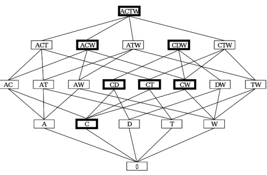
(29) 3.3 Frequent itemsets vs. frequent closed itemsets We show that how effective we use frequent closed itemsets. For example, Figure 4 describes all frequent itemsets and frequent closed itemsets on the lattice structure in this paper’s instance. If we focus on the item “A”, including “A” frequent itemsets are {A}, {AC}, {AT}, {AW}, {ACW}, {ACT}. {ATW}, {ACTW}, the total number of frequent itemsets containing “A” is 8. But frequent closed itemsets are only two {ACW}, {ACTW} The meaning of this fact is that if A exists in database and min_supp = 3, if we find transactions {1, 3, 4, 5}, we can discover the frequent closed itemsets “ACW”. Therefore we can obtain “ACW” all together with support count 4, i.e. maximal set of transaction {1, 3, 4, 5} is “ACW”. And we can find other items “CTW”. if we check transactions {1, 3, 5}, we can find the frequent closed itemsets “ACTW”. Therefore we can obtain “ACTW” with support count 3, i.e. maximal set of transaction {1, 3, 5} is “ACTW”. Totally apriori algorithm produced 19 itemsets, but if we use frequent closed itemsets only 7 itemsets. Therefore, We can reduce the number of frequency itemsets and we don’t lose frequency information in their datasets.. 23.

(30) ACTW. ACT. AC. AT. ACW. AW. A. ATW. CD. C. CDW. CT. CW. D. T. CTW. DW. TW. W. ０. Frequent itemsets. □;. Frequent closed itemsets □;. Figure3.2.Frequent itemsets VS Frequent closed itemsets on the lattice structure.. condition itemsets. frequent itemsets {A} {C} {D} {T} {W} {AC} {AT} {AW} {CD} {CT} {CW} {DW} {TW} {ACW} {CDW} {ACT} {ATW} {CTW} {ACTW}. total itemsets 19 itemsets. support_count 4 6 4 4 5 4 3 4 4 4 5 3 3 4 3 3 3 3 3. frequent closed itemsets. support_count. {C}. {CD} {CT} {CW}. 4 4 5. {ACW} {CDW}. 4 3. {ACTW}. 3. 7 itemsets. Table 3.1 frequent itemsets vs. frequent closed itmsets. 24.

(31) Chapter 4. Strong non-redundant association rules In this chapter we analyze definition of non-redundant association rules given by Lakhal, and based on this analysis we try to propose another form definition of non-redundant association rules. This definition called “strong non-redundant association rules”. Recall non-redundant association rules. As pointed out in example 4.1, it is desirable that only the non-redundant association rules with minimal antecedent and maximal consequent, i.e. the most useful and relevant rules, are extracted and presented to the user. Such rules are called non-redundant association rules.. 4.1 Lakhal’s definition vs. Strong definition Lakhal [4] considered, an association rule is redundant if it conveys the same information or less general information – than the information conveyed by another rule of the same usefulness and the same relevance. An association rule r ∈ E is non-redundant and minimal if there is no other association rule r '∈ E having the same support and same confidence, of which the antecedent is a subset of the antecedent of r and the consequent is a superset of the consequent of r . Definition 8 (Lakhal’s definition of non-redundant association rules) An association rule r : l1 → l 2 is a non-redundant rule, iff there does not exist an association rule r ' : l1' → l 2' with support(r) = support (r’), confidence(r) = confidence (r’), and l1' ⊆ l1 , l 2 ⊆ l 2'. 25.

(32) Example 4.1 We present an example of non-redundant association rules based on Lakhal’s definition [4]. Because our new definition basis his definition, so we present our basic concept of non-redundant association rules. This example extracted from UCI KDD’s archive’s datasets Mushroom [4]. These 9 rules have same support and same confidence. 1) Free gills →eatable 2) Free gills →eatable, partial veil 3) Free gills →eatable, white veil 4) Free gills, white veil →eatable 5) Free gills, partial veil →eatable 6) Free gills →eatable, partial veil, white veil 7) Free gills, partial veil →eatable, white veil 8) Free gills, white veil →eatable, partial veil 9) Free gills, partial veil, white veil →eatable Obviously, give rule 6, rule 1 to 5 and 7 to 9 are redundant, since they do not convey any additional information to the user. Rule 6 has minimal antecedent and maximal consequent and it is the most informative among these nine rules. But, our idea of non-redundant association rule is: “strong non-redundant association rules”. This leads to a definition of non-redundant association rules in strong, i.e. those satisfy the min_supp and min_conf. This definition says, “Compare all strong rules”. Noticing that Lakhal’s definition uses same support and same confidence, but our definition do not use same support and same confidence, we consider those with large or small support and confidence. Therefore our definition is Definition 9 (Strong non-redundant association rules) An association rule r : l1 → l 2 is a non-redundant rule, iff there does not exist an association. rule. r ' : l1' → l 2'. with. support(r) ≦ support(r’),. confidence(r’), and l1' ⊆ l1 , l 2 ⊆ l 2'. 26. confidence(r) ≦.

(33) The meaning of this definition, we consider that why people decrease min_supp, so we think everyone want to discover other rules. Therefore if we want to know the new rules in the strong space, then we do not need same information rules, in the strong space. So our new definition helps to discover other rules in the strong space. Our new definition can reduce non-informative rules, i.e. to reduce the non-informative rules in strong.. 4.2 Rules with confidence 100% The rules with confidence 100% of the form r : l1 → (l 2 \ l1 ), are rules between two frequent itemsets l1 and l 2 whose closures are identical: γ (l1 ) = γ (l 2 ) . Indeed, from γ (l1 ) = γ (l 2 ) we deduced that l1 ⊂ l 2 and support ( l1 ) = support ( l 2 ), and thus confidence ( r ) = 1. Since the maximum itemset among these itemsets is the itemset γ (l 2 ) , all supersets of l1 that are subsets of γ (l 2 ) have same support, and the rules between these two itemsets are rules with confidence 100%. Definition 10 (confidence with 100% rules based on Lakhal) Let FC be the set of frequent closed itemsets extracted from the context and, for each frequent closed itemset f , let denote G f the set of generators of f . Confidence with 100% rules = {r : g → ( f \ g ) | f ∈ FC ∧ g ∈ G f ∧ g ≠ f }. Definition 11 (confidence with 100% rules based on strong) Let FC be the set of frequent closed itemsets extracted from the context and, for each frequent closed itemset f , let denote G f the set of generators of f . Confidence with 100% rules =. {r : g → ( f \ g ) | f ∈ FC ∧ g ∈ G. f. ∧g ≠ f}. {r does not have r ' | g ⊇ g '∧( f \ g ) ⊆ ( f \ g )'∧ f . sup port > f '.sup port}. 27.

(34) The condition g ≠ f ensures that rules of the form g → 0 , which are non-informative, are discarded. The following proposition states that this definition.. Proposition 1.. (i). (ii). All valid confidence with 100% association rules, their supports and their confidences (that are equals to 100%) can be deduced from the rules of the generator, frequent closed itemsets and theirs supports. The generator and frequent closed itemsets basis for exact association rules contains only minimal non-redundant rules.. Proof･ Let r : l1 → (l 2 \ l1 ) be a valid confidence with 100% association rule between two frequent itemsets with l1 ⊂ l 2 . Since confidence(r) = 100% we have support ( l1 ) = support ( l 2 ) . Given the property that the support of an itemset is equal to the support of its closure, we deduce that support ( γ (l1 ) ) = support ( γ (l 2 ) ) → γ (l1 ) → γ (l 2 ) = f The itemset f is a frequent closed itemset f ∈ FC and, obviously, there exists a rule r ' : g → ( f \ g ) such that g is a generator of f for which g ⊂ l1 and g ⊂ l 2 . We show that the rule r and its support can be deduced from the rule r ' and its support. Since g ⊂ l1 and g ⊂ l 2 , the rule r can be derived from the rule r ' . From γ (l1 ) = γ (l 2 ) = f , we deduce that support ( r ) = support ( l 2 ) = support γ (l 2 ) = support ( f ) = support ( r ' ).. 28.

(35) Algorithm for constructing the generator and frequent closed itemsets basis Algorithm 4. Constructing the generator and frequent closed itemsets basis. Input: sets FCk of k-groups of frequent k-generators; Output: set GB of confidence with 100% association rules. 1) GB ~ {} 2) forall set FCk ∈ FC do begin 3) forall k-generator g ∈ FCk such that g ≠ γ (g) do begin 4). GB ~ GB U {(r : g → (, γ (g) \ g), γ (g)･support)};. 5) end 6) end 7) return GB; __________Lakhal’s definition stop 8) forall itemsets g ∈ GB and γ (g) \ g) ∈ GB 9) If { ¬∃ (g ⊇ g’) ∧ ¬∃ (( γ (g) \ g) ⊆ ( γ (g’) \ g’)) ∧ support ( γ (g) \ g) ≥ support ( γ (g’) \ g’)} then Strong{} ← g and ( γ (g) \ g) 11). end _____________Strong definition stop. The algorithm starts by initializing the set GB as the empty set (step 1). Each set FC k of frequent k-groups is then examined successively (steps 2 to 6). For each k-generator g ∈ FC k of the frequent closed itemset γ ( g ) for which g is different from its closure γ ( g ) (steps 3 to 5), the rule r : g ⇒ (γ ( g ) \ g ) , whose support is equal to the support of g and γ ( g ) , is inserted into GB (step 4). The algorithm returns the set GB containing non-redundant confidence with 100% association rules between generators and their closures in Lakhal’s definition (step 7). For all frequent itemsets generator and frequent closed itemsets in GB (step8). Step (9), if antecedent g does not have subset g’ in GB and consequent does not have superset (γ ( g ) \ g ) ’ in GB and these itemsets support are larger, input g and γ ( g ) to Strong {}.. 29.

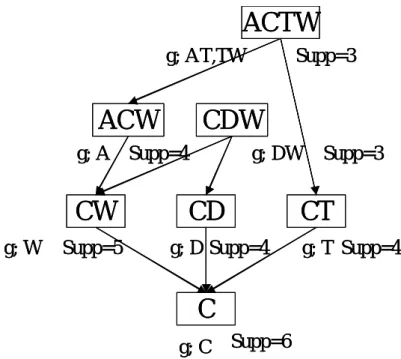
(36) Example 4. Rules based on Lakhal’s definition Confidence with 100% association rules extracted from the context D for a minimal support threshold of 3/6 is presented in Table 1. It contains 8 rules whereas 18 confidence with 100% association rules are valid on the whole.. ACTW g; AT,TW. CDW. ACW g; A Supp=4. g; DW Supp=3. CT. CD. CW g; W. Supp=3. Supp=5 g; D Supp=4. g; T Supp=4. C g; C. Supp=6. Figure4.1 generate rules on the lattice. FC1 generator {A} {C} {D} {T} {W}. closure {ACW} {C} {CD} {CT} {CW}. Sup_count 4 6 4 4 5. FC2 generator {AT} {DW} {TW}. closure {ACTW} {CDW} {ACTW}. Sup_count 3 3 3. generator closure rules on definition3 generator closure Lakhal's definition support_count {A} {ACW} A→CW A ACW A→CW 4 C {C} C {C} D {D} CD {CD}D→C D→Ｃ 4 T {T} CT {CT}T→C T→C 4 W{W} CW {CW}W→C W→C 5 AT{AT} ACTW AT→CW AT→CW 3 {ACTW} DW CDW DW→C 3 {DW} {CDW} DW→C TW TW→AC TW→AC 3 {TW} ACTW {ACTW}. Figure.4.2 Rules based on Lakhal’s definition. 30.

(37) Example 5. Strong definition Our definition recalculate the rules about antecedent and consequent, Lakhal’s definition produced 8 rules, but our Strong definition contain 5 rules.. generator A C D T W AT DW TW. closure ACW C CD CT CW ACTW CDW ACTW. Lakhal's definition A→CW. support_count 4. Strong definition A→CW. support_count 4. D→C D→C 4 T→C T→C 4 W→C W→C 5 AT→CW 3 DW→C 3 TW→AC TW→AC 3 Figure.4.3 lakhal definition vs. strong definition. 4 4 5 3. For example, DW→C in Lakhal’s definition, our definition does not produce it. Because compare to D→C, DW has subset D and C is equal to C and support count is lower, so our definition delete this rule.. 4.3 confidence with lower than 100% rules Each confidence with under100% association rule r : l1 → (l 2 \ l1 ) , is a rule between two frequent itemsets l1 and l 2 such that the closure of l1 is a subset of the closure of l 2 : γ (l1 ) ⊂ γ (l 2 ) . The non-redundant confidence with under 100% association rules with minimal antecedent l1 and maximal consequent (l 2 \ l1 ) are deduced from this characterization. Let f 1 be the frequent closed itemset which is the closure of l1 and g 1 a generator of f 1 such as g 1 ⊂ l1 ⊂ f 1 . Let f 2 be the frequent closed itemset which is the closure of l 2 and g 2 a generator of f 2 such as g 2 ⊂ l 2 ⊂ f 2 .The rule g 1 → ( f 2 \ g 1 ) between the generator g1 and the frequent closed itemset f 2 is the non-redundant rule among the rules between an itemset of the interval* [ g1 f 1 ] and an itemset of the interval [ g 2 , f 2 ]. Indeed, the generator g 1 is the minimal. 31.

(38) itemset whose closure is f 1 which means that the antecedent g 1 is minimal and that the consequent ( f 2 \ g 1 ) is maximal since f 2 is the maximal itemset of the interval [ g 2 , f 2 ]'. The generalization of this property to the set of all rules between two itemsets l1 and l 2 defines the informative basis which thus consists of all the non-redundant confidence with under 100% association rules of minimal antecedents and maximal consequents characterized. *The interval [ l1 l 2 ] contains all the supersets of l1 that are subsets of l 2 .. Definition 12 (Informative basis for confidence with under100% association rules). Let FC be the set of frequent closed itemsets and let denote G the set of their generators extracted from the context. The informative basis for confidence with under100% association rules is. IB = {r : g → ( f \ g ) | f ∈ FC ∧ g ∈ G ∧ γ ( g ) ⊂ f } . Proposition 2. (i) All valid confidence with under 100% association rules, their supports and confidences, can be deduced from the rules of the informative basis, their supports and theirs confidences. (ii) All rules in the informative basis are non-redundant confidence with under 100% association rules.. Proof. Let r : l1 → (l 2 \ l1 ) be a valid confidence with under100% association rule between two frequent itemsets with l1 ⊂ l 2 . Since confidence(r) < 1 we also have γ (l1 ) ⊂ γ (l 2 ) . For any frequent itemsets l1 and l 2 , there is a generator g 1 such that g 1 ⊂ l1 ⊂ γ (l1 ) = γ ( g 1 ) and a generator g 2 such that g 2 ⊂ l 2 ⊂ γ (l 2 ) = γ ( g 2 ) . Since l1 ⊂ l 2 , we have l1 ⊆ γ ( g 1 ) ⊂ l 2 ⊆ γ (g 2 ) and the rule r ' : g 1 → (γ ( g 2 ) \ g 1 ) belongs to the informative basis IB . We show that the rule r, its support and its confidence can be deduced from the rule r', its support and its confidence. Since g 1 ⊂ l1 ⊂ γ ( g 1 ) ⊂ g 2 ⊂ l 2 ⊂ γ (g 2 ) , the antecedent and the consequent of r can be. 32.

(39) rebuilt starting from the rule r'. Moreover, we have γ (l 2 ) = γ ( g 2 ) and thus support(r) = support ( l 2 ) = support ( γ ( g 2 ) ) = support ( r ' r'). Since g 1 ⊂ l1 ⊂ γ ( g 1 ) , we have support ( g 1 ) = support ( l1 ) and we thus deduce that: confidence(r) = support ( l 2 ) / support ( l1 ) = support ( γ ( g 2 ) ) / support ( g 1 ) = confidence ( r ' ) . From the definition of the informative basis we deduce the definition of the transitive reduction of the informative basis that is itself a basis for all confidence with under 100% association rules. We note l1 < l 2 if the itemset l1 is an immediate predecessor of the itemset l 2 , i.e. ¬∃l 3 such that l1 ⊂ l 3 ⊂ l 2 The transitive rules of the informative basis are of the form r : g → ( f \ g ) for a frequent closed itemset f and a frequent generator g such that γ ( g ) ⊂ f and γ ( g ) is not an immediate predecessor of fin FC FC: γ ( g )¬ < f . The transitive reduction of the informative basis thus contains the rules with the form r : g → ( f \ g ) for a frequent closed itemset f and a frequent generator g such as γ ( g ) < f . Definition 14 (Transitive reduction of the informative basis based on Lakhal). Let FC be the set of frequent closed itemsets and let denote G the set of their generators extracted from the context. The transitive reduction of the informative basis for confidence with under 100% association rules is: RI = {r : g → ( f \ g ) | f ∈ FC ∧ g ∈ G ∧ γ ( g ) < f } Definition 15 (Informative basis based on Strong). Let FC be the set of frequent closed itemsets and let denote G the set of their generators extracted from the context. The transitive reduction of the informative basis for confidence with under 100% association rules is:. r : g → ( f \ g ) |  RI =    f ∈ FC ∧ g ∈ G ∧ γ ( g ) < f ∧ g ⊇ g '∧( f \ g ) ⊆ ( f \ g )'∧ f . sup port > f '.sup port  Obviously, it is possible to deduce all the association rules of the informative basis with their supports and their confidences, and thus all the valid confidence with under100% rules, from the rules of this transitive reduction, their supports and their confidences. This reduction makes it possible to decrease the number of. 33.

(40) confidence with under 100% rules extracted by preserving the rules which confidences are the highest (since the transitive rules have confidences lower than the non-transitive rules by construction) without losing any information.. 34.

(41) Algorithm 5. Generating the transitive reduction of the informative basis. Input: sets FCk of k-groups of frequent k-generators; min_confidence threshold Output: Transitive reduction of the informative RI 1) RI ~ {} 2) for (k ← 1; k ≤ µ − 1; k + + ) do begin 3). forall k-generator g ∈ G do begin. 4). Succ g ← {};. 5). for ( j =| γ ( g ) |; j ≤ µ ; j + + ) do begin. 6) 7) 8) 9) 10). S j ← { f ∈ FC | f ⊃ γ ( g )∧ | f |= j}; end for ( j =| γ ( g ) ); j ≤ µ ; j + +) do begin forall frequent closed itemsets f ∈ S j do begin if (¬∃s ∈ Succ g | s ⊂ f ) then begin. 11). Succ g ← Succ g ∪ f ;. 12) 13). r.confidence ← f . sup port / g. sup port ; if (r.confidence ≥ min_ confidence);. 14). then RI ← RI ∪ {r : g → ( f \ g ), r.confidence, f . sup port};. 15) endif 16) end 17) end 18) end 19) end 20) return RI ; ________________________________ Lakhal’s definition stop 21) forall itemsets g ∈ RI and γ (g) \ g) ∈ RI 21) If { ¬∃ (g ⊇ g’) ∧ ¬∃ (( γ (g) \ g) ⊆ ( γ (g’) \ g’)) ∧ support ( γ (g) \ g) ≥ support ( γ (g’) \ g’)} then Strong{} ← g and ( γ (g) \ g) 22) end _______________________________________Strong definition stop. 35.

(42) The pseudo code of the Gen-RI algorithm for constructing the transitive reduction of the informative basis for the confidence with under 100% association rules using the set of frequent closed itemsets and their generators is presented in algorithm 5. Each element of a set FC k consists of three fields: generator, closure and. support. The algorithm constructs for each generator g considered a set Succg containing the frequent closed itemsets that are immediate successors of the closure of g.. The algorithm starts by initializing the set RI with the empty set (step l). Each set FC k of frequent k-groups is then examined successively in the increasing order of the values of k (steps 2 to 14). For each k-generator g ∈ FC k of the frequent closed itemset γ ( g ) . (steps 3 to 18), the set Succg of the successors of the closure of γ ( g ) is initialized with the empty set (step 4) and the sets S j of frequent closed j-itemsets that are supersets of γ ( g ) for | γ ( g ) |< j < µ *3 are constructed (steps 5 to 7). The sets S j are then considered in the ascending order of the values of j (steps 8 to 17). For each itemset f ∈ S j that is not a superset of an immediate successor of γ ( g ) in Succg (step 10), f is inserted in Succg (step 11) and the confidence of the rule r : g → ( f \ g ) is computed (step 12). If the confidence of r is greater or equal to the minimal confidence threshold minconfidence, the rule r is inserted in RI (steps 13 to 15). When all the generators of size lower than µ have been considered, the algorithm returns the set RI (step 20). *3 We denote, µ the size of the longest maximal frequent closed itemsets.. 36.

(43) ACTW g; AT,TW. CDW. ACW g; A Supp=4. CW g; W. Supp=5. Supp=3. g; DW. CD g; D Supp=4. Supp=3. CT g; T Supp=4. C g; C Supp=6 Figure 4.4 generate rules confidence with lower than 100%. generator. closure. closed superset. rules. support. confidence. A. ACW. ACTW. A→CTW. 75. 75. A. ACW. ACDW. A→CDW. 33.3. 50. C. C. CD. C→D. 66.7. 66.7. C. C. CT. C→T. 66.7. 66.7. C. C. CW. C→W. 83.3. 83.3. C. C. CDW. C. C. ACW. C. C. ACTW. D. CD. CDW. D→CW. 50. 75. D. CD. CDT. D→CT. 33.3. 50. T. CT. ACTW. T→ACW. 50. 75. T. CT. CDT. T→CD. 33.3. 50. W. CW. CDW. W→CD. 50. 60. W. CW. CWA. W→AC. 66.7. 80. W. CW. ACTW. AT. ACTW. ACDTW. AT→CDW. 16.7. 33.3. AD. ACDW. ACDTW. AD→CTW. 16.7. 50. DW. CDW. ACDW. DW→AC. 33.3. 66.7. DT. CDT. ACDTW. DT→ACW. 16.7. 50. TW. ACTW. ACDTW. TW→ACD. 16.7. 33.3. Table 4.1 generated rules confidence with lower than 100%. 37.

(44) Example 7 To compare Lakhal’s definition vs. Strong definition. Lakhal definition rules support confidence A→CTW 75 75 A→CDW 33.3 50 C→D 66.7 66.7 C→T 66.7 66.7 C→W 83.3 83.3 D→CW 50 75 D→CT 33.3 50 T→ACW 50 75 T→CD 33.3 50 W→CD 50 60 W→AC 66.7 80 AT→CDW 16.7 33.3 AD→CTW 16.7 50 DW→AC 33.3 66.7 DT→ACW 16.7 50 TW→ACD 16.7 33.3 total number of rules = 16. Strong definition rules A→CTW A→CDW C→D C→T C→W D→CW D→CT T→ACW T→CD W→CD W→AC. TW→ACD. support confidence 75 75 33.3 50 66.7 66.7 66.7 66.7 83.3 83.3 50 75 33.3 50 50 75 33.3 50 50 60 66.7 80. 16.7. 33.3. total number of rules = 12. Figure4.5 Lakhal’s definition vs. strong definition. 38.

(45) Chapter5 Efficient algorithm to generate non-redundant association rules In this chapter we investigate the definition of non-redundant association rules given by Zaki. We present an efficient algorithm to generate non-redundant association rules that definition.. 5.1 Minimal antecedent and minimal consequent An association rule is form of the l1 → l 2 , where l1 , l 2 ∈ I . Its support equals γ (l1 ∪ l 2 ) , and its confidence is given as conf = P (l1 | l 2 ) =| γ (l1 Υ l 2 ) | / | γ (l1 ) | . We are interested in finding all high support and confidence rules, i.e. rules satisfy the min_supp and min_conf. It is widely recognized that the set of such association rules can rapidly grow to e unwieldy. In this chapter we will show the frequent closed itemsets help us form a generating set of rules, from which all other association rules can be inferred. Thus, only a small and understandable set of rules can be presented user, who can later selettively derive other rules of interest.. 39.

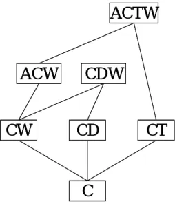
(46) Definition (Zaki’s definition of non-redundant association rules) An association rule r : l1 → l 2 , We say that a rule r is more general than a rule. r ' : l1' → l 2' , denoted r ≤ r ' provided that r’ can be generated by additional items to either the antecedent or consequent of r. Let R = {R1 Λ , Rn } be a set of rules, such that all their confidence are equal. Then the non-redundant rules in the collection R are those that are most general, with support(r) = support (r’), confidence(r) = confidence (r’), and l1' ⊆ l1 , l 2 ⊆ l 2' This definition indicates that minimal antecedent and minimal consequent association rules are non-redundant association rules.. ACTW. ACW. CW. CDW. CD. CT. C Figure 5.1 frequent closed itemsets lattice. We show how to eliminate the redundant association rules, i.e. rules having the same support and confidence as some more general rules. In this section, we showed that the support of an itemsets l equals the support of its closure γ (l ) . Thus it suffices to consider rules only among the frequent closure itemsets. In other words the rule r : l1 → l 2 is exactly the same as rule r : γ (l1 ) → γ (l 2 ) .. 40.

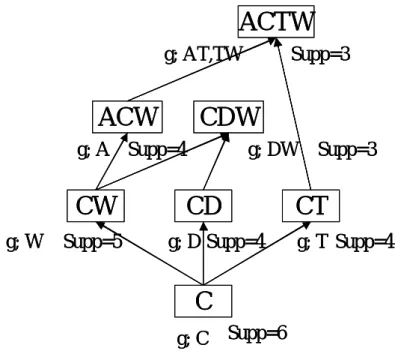
(47) Another observation that follows from the frequent closed itemsets lattice is that sufficient to consider rules among adjacent frequent closed itemsets, since other rules can be inferred be transitivity, that is Lemma transitivity Let l1 l 2 l3 be frequent closed itemsets, with l1 ⊆ l 2 ⊆ l3 . If l1 → l 2 (conf = p ), and l 2 → l 3 (conf = q) then l1 → l3 (conf = p * q). 5.2 Rules with confidence 100% In this section, we consider the how to generate confidence with 100% rules.. Lemma (confidence with 100% rule) An association rule l1 → l 2 confidence =100%, if and only if γ (l1 ) ⊆ γ (l 2 ) . This theorem says that all 100% confidence rules are those that are directed from super frequent closed itemsets to a sub frequent closed itemsets.. ACTW Supp=3. ACW. CDW. Supp=4. CW Supp=5. Supp=3. CD. CT. Supp=4. Supp=4. C Supp=6 Figure 5.2 rules based on original theorem. 41.

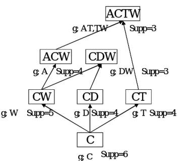
(48) For example frequent closed itemsets CW and C, the rule W→C is a 100% confidence rule. Note that if we take the closure on both sides of rule, we obtain CW → C, i.e. a rule between closed itemsets, but since the antecedent and consequent are not disjoint in this case, we prefer to write the rule as W→C, although both Theorem 1. Let R = {R1 Λ , Rn } be a set of rules with 100% confidence rules, such that I 1 = γ (l1 Υ l 2 ) and I 2 = γ (l 2 ) for all the rules Ri ≠ RI are more special than R I ,. and thus are redundant. But we noticed what mean of this theorem, in chapter 3, we showed that the support of. an itemset l1 equals to the support of its closure γ (l1 ) and its generator g. Therefore it suffices to consider rules only among the frequent closed itemsets. Thus most minimal itemsets is generator, so we can generate rules directly generator to generator, instead of closure items.. ACTW g; AT,TW. CDW. ACW g; A Supp=4. CW g; W. Supp=5. Supp=3. g; DW. CD g; D Supp=4. Supp=3. CT g; T Supp=4. C g; C Supp=6 Figure 5.3 rules based generator. 42.

(49) 5.3 confidence with lower than 100% rules We now turn to problem of finding a generating set for association rules with confidence less than 100%. As befor, we need to consider only the rules between adjacent frequent closed itemsets.. Theorem Let R = {R1 Λ , Rn } be a set of rules with confidence p < 1.0 , such that I 1 = γ (l1 ) and I 2 = γ (l1 Υ l 2 ) for all rules Ri . Let R I denote the rule I 1 → I 2 . Then all the rules Ri ≠ RI are more specific than R I , and thus are redundant.. This theorem differs from that of the 100% confidence rules to account for the up arc.. ACTW Supp=3. ACW. CDW. Supp=4. CW Supp=5. Supp=3. CD. CT. Supp=4. Supp=4. C Supp=6. Figure 5.4 Rules based on original theorem For example frequent closed itemsets C and CW, the rule C→W is a rule with less than 100% confidence. Note that if we take the closure on both sides of rule, we. 43.

(50) obtain CW→C, i.e. a rule between closed itemsets, But we noticed what mean of this theorem, in chapter 3, we showed that the support of. an itemset l1 equals to the support of its closure γ (l1 ) and its generator g. Therefore it suffices to consider rules only among the frequent closed itemsets. Thus most minimal itemsets is generator, so we can generate rules directly generator to generator, instead of closure items. In this case, i.e. confidence less than 100% we can generate the rules, generator W comes from frequent closed itemsets CW to generator C comes from frequent closed itemsets C. So we can generate rule directly. Thus our method is effective.. ACTW g; AT,TW. ACW. CDW. g; A Supp=4. CW g; W. Supp=5. Supp=3. g; DW. CD. Supp=3. CT. g; D Supp=4. g; T Supp=4. C g; C. Supp=6. Figure 5.5 Rules based generator. 44.

(51) Chapter 6 Experimentals In this section we describe experimental environments and results. So we try to visualize my definition of non-redundant association rule is more effective.. 6.1 Experimental design Our experiments are three categories. First we try to compare how effective Lakhal’s definition, so we try to compare Apriori vs. Lakhal’s algorithm. Second we try to how effective our new definition, so we try to compare Lakhal’s algorithm vs. Strong algorithm. Finally we compare three algorithms. Datasets We used the 10 datasets during these experiments comes from UCI datasets. name. number of items number of transactions. 1. sample. 5. 6. 2. corral. 7. 31. 3. muxf6. 7. 63. 4. party. 11. 101. 5. tutrial. 11. 10. 6. lenses. 12. 16. 7. golf. 14. 14. 8. Co2. 14. 31. 9. mux. 14. 63. 10. led7. 16. 200. 11. hungarian. 17. 196. 12. Monk1. 19. 124. 13. monk2. 21. 169. Table 6.1 datasets. 45.

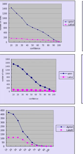
(52) 6.2 Experimental results 6.2.1 apriori vs. Lakhal’s algorithm In this part we present the result of experimental to compare Apriori to Lakhal’s definition. Generated rules of Lakhal’s definition are all times smaller than Arioiri. Specially if threshold of support i.e. min_supp is small, then generated rules are very small, Lakhal’s definition is more effective in this case, i.e. if min_supp is small then Apriori produced many redundant rules. 1600. 70. 1400. 60 number of rules. number of rules. 1200 1000 apriori Lakhal. 800 600 400. 50 40. 20 10. 200. 0. 0 10. number of rules. apriori Lakhal. 30. 20. 30. 40. 50 60 70 confidence. 80. 90. 10. 100. 1800. 500. 1600. 450. 1400. 400. 20. 30. 40. 50 60 70 confidence. 80. 90. 100. 350. 1200 1000. apriori. 300. 800. Lakhal. 250. 600. 200. 400. 150. 200. 100. 0 10. 20. 30. 40. 50. 60. 70. 80. apriori Lakhal. 50. 90 100. 0. confidence. 10. 20. 30. 40. 50. 60. 70. 80. 90 100. 450 400 350 300 250. Apriori Lakahl. 200 150 100 50. Figure 6.1 Apriori vs. Lakhal algorithm. 90 10 0. 70. 80. 60. 50. 40. 30. 20. 10. 0. 46.

(53) 6.2.2 Lakhal’s algorithm vs. strong algorithm. In this part, we present the result of experimental to compare Lakhal’s definition to new definition “Strong non-redundant association rule”. We present two cases result, our new definition is more effective case and the other is same result of total number of generated rules. Almost experiments, our strong definition can reduced the number of rules, but some time the result is equal to previous work.. 100. 18. 90. 16. 80. 14. number of rules. 70. 12. 60 Lakhal Suzuki. 50. 10. 40. Lakhal Strong. 8. 30. 6. 20. 4. 10. 2. 0 10. 20. 30. 40. 50. 60. 70. 80. 90. 0. 100. 10. confidence. 50. 20. 30. 40. 50. 60. 70. 80. 90 100. 70. 45 60 50. 35 number of rules. number of rules. 40. 30 Lakhal Suzuki. 25 20 15. 40. Lakhal Suzuki. 30 20. 10 10. 5. 0. 0 10. 20. 30. 40. 50 60 70 confidence. 80. 90. 10. 100. 20. 30. 40. 50. 60. 70. 80. 90. confidence. 180 160 140 120 100. Lakhal Strong. 80 60 40 20 0 10. 20. 30. 40. 50. 60. 70. 80. 90 100. Figure 6.2 Lakhal vs. strong. 47. 100.

(54) Chapter 7 Conclusion Finally we conclude this paper. Recall, Our research has four objectives. 1. To investigate the problem of non-redundant association rules. 2. To try to formulate another form of non-redundant association rules. 3. To develop an algorithm that finds non-redundant association rules. 4. To try to improve the algorithm. The frequent closed itemsets helps us to produce non-redundant association rules in chapter 3. If we use frequent closed itemsets, so we can reduce redundant itemsets. About first objective, We discus chapter 3,4 and 5, two definition exist in previous works, to generate minimal antecedent and maximal consequent rules can deduce the other rules. About second objective and third objective, we try to develop new definition of non-redundant association rule in chapter4. We experiments in chapter6This definition generate smaller size rules than Lakhal’s definition; we do some experiments in chapter 6. About fourth objective, we did not experiment, but obviously my algorithm is efficiently, because Zaki, produced all candidate rules, the after to select most general rule, but my algorithm can generate most general rule directly. So it may the cost of calculation is lower than original algorithm. Finally we cannot say when or which time to use which algorithm. But we investigate all definition of previous and our non-redundant association rules, so. 48.

(55) if we analyze some datasets, our research help people who want to discover new knowledge by association rule mining.. 49.

(56) Acknowledgement First of all, I would like to express profoundly my appreciation to Professor Tu Bao Ho for his a lot of kindness, patience and effectual support during the work. And Professor Masato Ishizaki in knowledge creating Laboratory, Professor Yoshiteru Nakamori and Kenji Satou they give some comment in middle examination. And Ngyuyen Trong Dung, Saori Kawasaki, Toyohisa Nakada, and Matunaga, they help me to do programming, and some commends. Thank you very much for everyone.. References [1] R. Agrawal, T. Imielinski, A. Swami: "Mining Associations between Sets of Items in Massive Databases", Proc. of the ACM-SIGMOD 1993 Int'l Conference on Management of Data, Washington D.C., May 1993, 207-216. [2] R. J. Bayardo Jr. Efficiently Mining Long Patterns from Databases. In Proc. of the 1998 ACM- SIGMOD Int'l Conf. on Management of Data, 85-93, 1998. [3] R. J. Bayardo Jr. and R. Agrawal, "Mining the Most Interesting Rules" In Proc. of the 5th ACM SIGKDD Int'l Conf. on Knowledge Discovery and Data Mining, August 1999. Expanded version available as IBM Research Report RJ 10146, July 1999. Abstract.. 50.

(57) [4] Y. Bastide, N. Pasquier, R. Taouil, G. Stumme, L. Lakhal "Mining Minimal Non-Redundant Association Rules using Frequent Closed Itemsets" 6th International Conference on Deductive and Object-Oriented Databases (DOOD-2000) 1st International Conference on Computional Logic (CL- 2000), Lecture Notes in Computer science, Springer-Verlag, Imperial College, London (UK), July 24-28, 2000. [5]S. Lopes, J.-M. Petit, L. Lakhal "Efficient Discovery of Functional Dependencies and Armstrong Relations" research report, Université Blaise Pascal - Clermont-Ferrand II, 1999. [6]Mohammed J. Zaki, Ching-Jui Hsiao, CHARM: An Efficient Algorithm for Closed Association Rule Mining, RPI Technical Report 99-10, 1999. [7]Mohammed J. Zaki, Generating Non-Redundant Association Rules, 6th ACM SIGKDD International Conference on Knowledge Discovery and Data Mining, pp 34-43, Boston, MA, August 2000 (also as RPI Technical Report 99-12).. [8] Nicolas Pasquier Yves Bastide Rafik Taouil Lotif Lakhal Closed set Based Discovery of small Covers for association Rules,1999. [9] Jiawei Han Micheline Kamber Data Mining Morgan Kaufmann publishers. [10] N.pasqire, Y. bastide, R.Taouil, and L. Lakhal. Pruning closed itemset lattice for association rule. Proc.BDA conf., pp 176-196, October 1998. [11] D. Heckerman. Bayesian networks for knowledge discovery. Advances in knowledge discovery and data mining, pp273- 305 1996. 51.

(58) [12] G. Piatetsky-Shaprio and C.J. Matheus. The interestingness of deviations. AAAI KDD workshop, pp25-36, july 1994. [13] A. Silberschatz and A. Tuzhilin. What makes patterns interesting in knowledge discovery systems. IEEE Transactions on knowledge and data Engineering, 8(6):970-974, December 1996. [14] B. Ganter and R. Wille. Found Concept Analysis: Mathmatical foundations. Springer, 1999. 52.

(59) 53.

(60)