A Multi-generation Product Diffusion Model
with Social Media Effects -Accerelating Effect
of Social Media on Leapfrogs and Switches by
the iPhone 6 Battery Problem 2016
2017-著者
Li Yinxing, Terui Nobuhiko
journal or
publication title
DSSR Discussion Papers
number
107
page range
1-39
year
2020-02
URL
http://hdl.handle.net/10097/00127167
Data Science and Service Research
Discussion Paper
Discussion Paper No. 107
A Multi-generation Product Diffusion Model with Social Media Effects
-Accerelating Effect of Social Media on Leapfrogs and Switches
by the iPhone 6 Battery Problem 2016–2017 - Yinxing Li and Nobuhiko Terui
February, 2020
Center for Data Science and Service Research Graduate School of Economic and Management Tohoku University 27-1 Kawauchi, Aobaku Sendai 980-8576, JAPAN
A Multi-generation Product Diffusion Model with Social Media Effects
-Accerelating Effect of Social Media on Leapfrogs and Switchesby the iPhone 6 Battery Problem 2016–2017 -
Yinxing Li and Nobuhiko Terui1
Graduate School of Economics and Management Tohoku University
Sendai, Japan
February, 2020
1 Tohoku University, Graduate School of Economics and Management, Kawauchi Aoba-ku,
Sendai, 980-8576, Japan. [email protected]; [email protected]
Terui acknowledges a grant by JSPS KAKENHI Grant Number (A)17H01001. Li acknowledges a grant by JSPS KAKENHI Grant-in-Aid for Research Activity start-up 19K23187.
A Multi-generation Product Diffusion Model with Social Media Effects
-Accerelating Effect of Social Media on Leapfrogs and Switchesby the iPhone 6 Battery Problem 2016–2017 -
Abstract
This paper proposes a multi-generational model that captures the direct and indirect ef-fects of social media on product diffusion. Direct efef-fects appear in the adoption rate function as covariates, and indirect effects are imbedded in hierarchical models connect-ing diffusion parameters to successive generations. Unlike previous multi-generational diffusion models, ours forecasts sales of new-generation products before launch using social media as the leading indicator and a hierarchical model connecting successive diffusion parameters. Empirical results show our model forecasts more precisely and re-veals how social media influenced sales of smartphones, particularly leapfrogging and switching to other generations and competing products, as Apple contended with defec-tive batteries in the iPhone 6 during 2016–2017.
1. Introduction
Frameworks of diffusion studies generally follow the Bass (1969) model that assumes a social network is homogeneous and fully connected and that new adopters enter the mar-ket influenced by innovators and producers' marmar-keting communications. Studies tradi-tionally attribute the internal effect to the influence of word of mouth.
Peres et al. (2010) trace how diffusion studies since 1990 have transitioned from inter-personal communication (Mahajan, Muller, and Bass, 1990; Mahajan and Wind, 2000) to more general interactions, including social interdependence (Goldberg and Lilien, 2010; Van den Burte and Lilien, 2001).
Diffusion of multi-generational products also has been investigated using the Bass model by connecting single-generation models sequentially. Since Norton and Bass (1987) proposed a diffusion model applicable to successive generations, many studies, including Mahajan and Muller (1996) and Jiang and Jain (2012), have extended it to multi-generational diffusions using sales and marketing mix data during the initial pe-riod after launch.
Alongside such data, this study incorporates data from consumers communicating over social media and proposes a multi-generational diffusion model that detects the ef-fects of social media before and after a product launches. It advances the literature in several respects. First, our model uses data other than post-launch sales to track diffu-sion of new products. In addition to price and competitors featured in the extended Bass models in Von Bertalanffy (1957), Mahajan and Muller (1981), Eastingwood et al. (1983) and Bewley and Fiebig (1988), we construct covariates by extracting text fea-tures from social media and incorporating them as social media effects into the adoption
rate function of a multi-generational diffusion model, implying the direct effect of social media.
Second, earlier diffusion models assume that key parameters of market potential and imitation rates are independent among generations when the innovator parameter is given. Our model structures generation-specific parameters hierarchically to depict the mecha-nism underlying parameter shifts between generations. Our structural model of parameter shift across generations facilitates forecasting sales of new-generation products before launch. The term of social media effect is incorporated in the hierarchical models and it affects indirectly to sales.
Third, our model measures the effects of social media on sales, particularly leapfrogs and switches, by the defective battery problem that plagued the iPhone 6 since early No-vember of 2016 and it became a hot topic in social media until the late of 2017. This “Battery Problem” is explained in detail in section 5. To measure this effect, we propose a labeled dynamic topic model as a hybrid of the labeled topic model (Daniel et al., 2009) and the dynamic topic model (Blei and Lafferty, 2006). Our model employs “battery” a
priori as the specific dynamic topic that captures the shift in distribution of topics over
time. We show empirically that social media reactions to iPhone's battery problem accel-erated switching and leapfrogging to later-generation iPhones and competing products.
Section 2 discusses the effects of social media on multi-generational diffusion. Section 3 explains our model. Section 4 reveals empirical results for sales of successive genera-tions of iPhones and shows our model predicts sales of products pre-launch by recogniz-ing social media effects. Section 5 shows the acceleratrecogniz-ing effects of the iPhone 6 battery problem on leapfrogging and switching to later-generation iPhones and competing phones. Section 6 concludes.
2. Social Media Effects and Diffusion
2.1 Multi-generational Diffusion Model
Research into the diffusion of product generations adopts the framework of multi-gener-ational diffusion models. The main differences among earlier models are their assump-tions about key parameters and their use of marketing mix variables. Among studies dis-tinguished by their key parameters, Norton and Bass (1987) assume that market potential
m for a generation of product depends on innovation and imitation parameters p and q are
constant across generations. Mahajan and Muller (1996), Jun and Park (1999), Kim et al. (2000), Danaher et al. (2001), and Jiang and Jain (2012) assume the constancy of p across generations, generation-specific market potential, and imitation parameters. Jiang (2010) and Guo and Chen (2018) assume that all parameters vary across generations.
Among diffusion studies distinguished by marketing mix variables, Robinson and Lakhani (1975) insert a price effect term into the adoption rate function, and Bass (1980) introduces price effects. These studies show that incorporating price information im-proves model performance. Horsky and Simon (1983) incorporate an advertising variable directly into sales, not into adoption rate function, and Horsky (1990) incorporates jointly advertising and price information.
The adoption rate function in Bass et. al (1994) includes two marketing mix variables: rates of change in prices and advertising expenditures relative to expenditures at product launch. Doing so permits comparing the effects of marketing variables. Jiang and Jain (2012) extend this model to a multi-generational diffusion model.
2.2 Labeled Dynamic Topics on Social Media
Marketing studies consider the effects of social media by extracting latent topics and their features from large-volume documents and modeling them as covariates. Natural
language processing is noteworthy in this regard, as indicated by the Latent Dirichlet Al-location (LDA) model of Blei et al. (2003).
Recent research uses topic models to analyze text data for marketing applications. The LDA model of Tirunillai and Tellis (2014) incorporates consumer reviews into five sets of marketing data to extract dimensions (topics) from UGC (User Generated Content) for comparison among markets. They find that some topics resonate across multiple markets and others only in certain markets. Through sentimental analysis they tag topics for better interpretation and show that multidimensional scaling via LDA captures the dynamics of brand positioning. Netzer et al. (2012) exploit the co-occurrence of words and semantic network analysis to derive market structure from online consumer forums. Their study highlights use of text mining to indicate marketing effectiveness and how marketers can affect brand position.
Li and Terui (2018) incorporate social media effects into a diffusion model to discuss how they influence market potential and internal parameters. Analyzing text data of SNS on mobile phones, they extract subjective and objective features by naïve Bayes and topic analysis respectively, then use them as covariates of time-varying market potential and imitation parameters. They show how social media affect single-generation diffusion of mobile phones and enhance forecasts. The supervised topic model of Ansari et al. (2018) identifies topics hidden in product reviews that reveal consumer preferences. Their sto-chastic variational Bayesian approach yields fast and scalable inferences from big data.
The dynamic topic model (DTM) is a generative model that reveals the evolution of topics hidden in collections of documents. Blei and Lafferty (2006) extend the LDA model to a dynamic model for handling sequential documents. They describe the
dynam-{
θt k, ,k=1,...,K−1}
and vocabulary distribution with parameters{
ψt k, ,t=1,...,K−1}
ina state space model so that they have a shift in the mean of Gaussian distribution when the previous state is given. That is, they assume that parameters shift as follows:
(
)
(
)
1 1 1 1 2 , , , 2 | , , | , . t t t t t t k k k h h N h h h N h θ θ θ θ ψ ψ ψ ψ σ σ − − − − (3.1)Corresponding to latent topics in the DTM, our study identifies topics on social media and enters them into our multi-generational diffusion model to uncover changes in con-sumer’s interests.
Next, focusing on the social media coverage following iPhone's battery problem, we extend the DTM by labeling one topic “battery.” Daniel et al. (2009) extend the LDA model by labeling topics to be estimated in advance. We extend their labeled topic model to a labeled dynamic topic model (LDTM), which is characterized as a hybrid of the la-beled topic and DTMs. Its graphical representation appears in the Appendix.
We denote 𝜂𝜂 as the hyper parameter for the prior probability that some specific words
include “battery” among three topics. Then we define 𝜂𝜂”𝑏𝑏𝑏𝑏𝑏𝑏𝑏𝑏𝑏𝑏𝑏𝑏𝑏𝑏” = (1, 0, 0) to indicate all instances of “battery” are bound to the first topic when assigned in the MCMC procedure. Other words are allocated as per DTM.
3. Models
3.1 Direct Effects of Social Media on Multi-generational Diffusion
We employ the sales function in Srinivasan and Mason (1986) to define our multi-gener-ational diffusion model. Norton and Bass (1987) proposed a successive-generations
Jiang and Jain (2012) that assumes p is constant across generations but q as well as market potential m are generation-specific.
First, we denote y t as the G-th generation adoptions at time t with launch timeG( ) 𝜏𝜏𝐺𝐺 > 0, and then following Jiang and Jain (2012), we define our model with additive noise for adoption of each generation as follows: Starting with the first generation launched at time 0, we have
(
)
(
)
1 1 1 1 2 1 1 1 2 2 1 2 1 ( ) ( ) ( ), , ( ) ( ) 1 ( ), , ( ) ( ) ( ) ( ) ( ), , 1 , G G G G G G G y t m f t u t t y t m f t F t u t t y t I t L t S t u t t G N τ τ τ τ τ + = + < = − − + ≥ = + + + ≤ < < ≤(
)
(
)
(
)
(
)
(
)
(
)
(
)
1 1 1 1 1 1 1 1 ( ) ( ) ( ) ( ) ( ) ( ) ( ) ( ) ( ) ( ) ( ), , 1 , ( ) ( ) ( ) ( ) 1 ( ), G G G G G G G G G G G G G G G G G G G G G G G G G G G G G G G G G m f t F t y t F t Y t f t u t y t I t L t S t L t u t t G N m f t F t y t F t Y t f t F t u t τ τ τ τ τ τ τ τ τ τ − − + + − − + + ≡ − − + − + − + = + + − + ≥ < ≤ ≡ − − + − + − × − − + (3.1) where I t is the independent adoption of the G-th generation, G( ) Y t denotes cumula-G( )
tive adoptions (sales) of the G-th generation at time t, fG=FG
( )
t −FG(
t− , and ( )1)
L t Gand SG( )t are adoptions from leapfrogging and switching, respectively.
In Eq.(3.1), the error term u t is assumed to follow normal distribution G( )
(
2)
( ) 0,
G
u t N σ independently across generations and time. We assume constant
vari-ance across generations because our data do not identify sales by generation. The adoption
rate function FG
( )
t for the G-th generation product accommodates not only marketingmix according to Jiang and Jain (2012) but also social media effects :
( )
(1 exp)(
((
( ) )( ))
)
1+ exp ( ) = G G G G G G p q X t q / p p q X t F t − − + − + , (3.2)(
)
( ) log ( ) (0) ' ( 1) ( ).
G G G G G G x
X t = +t β V t V +α LTopic t− +e t (3.3) In the above, VG( )t is the price of the G-th generation product in period t and β is the G
coefficient of the price effect. LTopicG(t−1) is a K dimensional vector with the element of log
(
TopicGi(t−1) TopicGi(0))
, whereTopicGi(t− denotes the frequency of words 1) in the i-th topic at t− , and 1 α is the corresponding coefficient vector. We assume that Gerror term e t follows x( ) .
We use 𝑇𝑇𝑇𝑇𝑝𝑝𝑇𝑇𝑇𝑇𝐺𝐺𝐺𝐺(𝑡𝑡 − 1) rather than 𝑇𝑇𝑇𝑇𝑝𝑝𝑇𝑇𝑇𝑇𝐺𝐺𝐺𝐺(𝑡𝑡) to acknowledge the leading property of the social media effect, i.e., people chat before they act. Social media variables usually are leading indicators of sales in related research (Li and Terui, 2018), and we show it is empirically confirmed for our data in section 4.
3.2Indirect Effects of Social Media via Generation-Specific Parameters
We assume that diffusion in each generation persists from the previous generation. Spe-cifically, generation-specific parameters are determined by those of previous generations, and topics 𝑻𝑻𝑮𝑮 are defined as the vector of number of words allocated to each topic after the G-th generation launch for 𝑡𝑡 < 𝜏𝜏𝐺𝐺 . If we denote TopicG( )t =
(
TopicG1( ),...,t TopicGK( ) 't)
, then T is represented byG ( )G G
t<τ t
∑
Topic .Then we define the structural equations for 𝑚𝑚𝐺𝐺 and 𝑞𝑞𝐺𝐺 as
0 1 1 0 1 1 0 1 1 0 1 1 ' ' ' ' ' , G m m G mT G m G q q G qT G q G G T G G G G m m q q α α α α β β β β δ δ ε δ δ ε δ ε β δ δ β ε − − − − = + + + = + + + = + + + = + + + δ T δ T α δ T δ T δ α (3.4)
(
2)
( ) 0, x x e t N σwhere we assume
(
2)
0,i N i
ε σ for the i-th equation and independence across equations.
These models define prior distributions for the parameter and we constitute the posterior distributions when combined with the likelihood function derived by Eqs. (3.1)–(3.3).
Jiang and Jain (2012) use the data of number of units and the aggregate adoption sales with marketing variables. However, their empirical performance is undemonstrated be-cause their marketing mix data are unavailable. We also find that estimated parameters of multi-generations are unstable when the number of generations increased. Further-more, models by Jiang and Jain (2012) and Norton and Bass (1987) structurally do not allow forecasting next-generation sales before launch because they lack structure to con-nect generations for parameters. Our hierarchical model in Eq.(3.4) accommodates pa-rameter shifts from previous generations and social media effects on papa-rameters.
3.3 Posterior Density for Model Parameters
The joint posterior density of our model parameters is represented by
{
} {
}
{
} {
}
{
} {
}
(
)
{
} { } {
}
{
}
{
}
(
)
(
{
} {
}
)
{
}
(
)
{
}
(
)
{
}
G G G G , , , , , , , , , , , , , , | , , , , = , , , | , , , , , , | , , , , , | , , , , , | , , , , , | , , , , G G G x m q G G G G G G G G G G G G G G G G G x G G G x x G G G p m q p t p m q p X t p m q p t X p X t p X t p X t β σ β σ σ σ σ β σ σ σ β σ σ β × × m q α β α m q α β Δ Δ Δ Δ σ Δ Δ α α Δ Δ α α y LTopic T V y y LTopic V LTopic V(
{
LTopic}
)
{
} { }
(
)
(
{
} { }
)
{
} { }
(
)
(
{
} { }
)
{
} { }
(
)
(
{
} { }
)
{
} { }
(
)
(
{
} { }
)
1 1 1 1 1 1 1 1 , | , , , | , , , | , , , | , , , | , , , | , , , | , , , | , , , (3.5) G G G G m m G G G G G G q q G G G G G G G G G G G G G G G p m m p m m p q q p q q p p p β p β σ σ σ σ α α α α β β σ σ β β − − − − − − − − × × × × m m q q α α α α β β Δ Δ Δ Δ Δ σ σ Δ Δ Δ V T T T T T T T TThe second line of (3.5) captures the product of conditional posterior density for pa-rameters in the diffusion model in Eqs. (3.1) and (3.2). The third and fourth lines are joint posterior density of parameters in the marketing mix in Eq. (3.3). The fifth to eighth lines define joint posterior density for parameters in the hierarchical structure connecting the (G-1) generation to the G generation in Eq.(3.4).
We employ MCMC to estimate parameters because the procedure for hierarchical models is well-established and some of necessary conditional posterior densities are available in closed form. The sampling scheme of MCMC for estimating the model is a hybrid of Metropolis-Hastings and Gibbs sampling for other parameters in hierarchical models. The algorithm appears in the Appendix.
3.4 Predictive Density
According to Eqs. (3.1) and (3.2), if we simulate sales for the second-generation product, we need at least one data point of that generation to estimate 𝑚𝑚2 and 𝑞𝑞2 even when 𝑝𝑝 is assumed constant across generations. 𝜶𝜶𝟐𝟐 and 𝛽𝛽2 also must be estimated using data for the second generation. The feature of their models hampers forecasting new generations with-out numerical data for this generation.
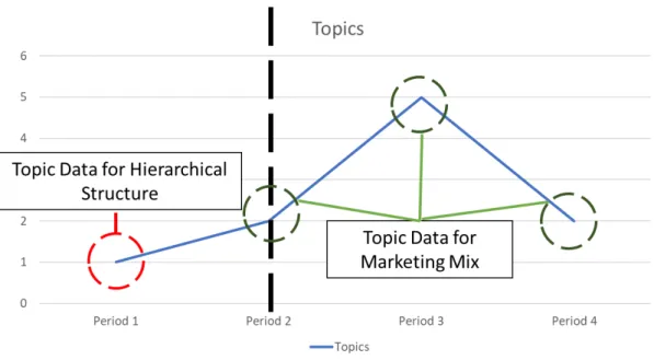
Fig. 3.1 Role of Social Media Pre- and Post-Launch
We note that the topic’s total frequency vector (𝑻𝑻𝑮𝑮) in Eq. (3.4) differs from vector 𝑳𝑳𝑻𝑻𝑻𝑻𝑻𝑻𝑻𝑻𝑻𝑻𝐺𝐺(𝑡𝑡 − 1) in Eq. (3.3), as Fig 3.1 exemplifies. Before G-th generation launches,
only social media provide information about a new generation of G-th product. Then, in terms of hierarchical models in Eq. (3.4) implying prior information, we forecast adoption of new generations when parameters are given. After G-th generation product launches,
the marketing mix (Eq. (3.3)) enters the adoption rate function to generate the forecast. Two structures using social media make it possible to use text data fully and to compare social media effects before and after new generations launch. Forecasting is constituted formally by the predictive density.
(
)
(
) (
)
(
) (
)
(
)
(
)
1 1 1 1 1 1 ( ) | , , , ( ), , ( 1), ( ) ( ) | , , , , , | , , ( ) | , , , ( ) , , | , , ( ) | , , , ( 1), ( ) , | , ( ) G G G G G G G G G G G G G G G G G G G G G G G G G G G G G G G G G G G G G G p y t m q p X t t V t p y t m q p t p m q p m q dm dq dp if t p y t m q p X t p m q p m q p X t t t V t p dX t τ β β β − − − − − − − = ≤ = × − ×∫
∫
T LTopic T T LTopic ,T α α α dm dq dG G αGdβGdp if t >τG (3.6)These integrations are numerically evaluated in the MCMC iterations as were applied to time series forecasting by Terui et al. (2010) and Terui and Ban (2014). The algorithm for Eq.(3.6) appears in the Appendix.
4. Empirical Results
4.1 Data
We use five generations of iPhone products with the same launching times between iPhones 5 through 7 as training data, .i.e., G1(iPhone 5), G2(iPhone 5s, 5c), G3(iPhone 6, 6 Plus), G4(IPhone 6s, 6s Plus), G5(iPhone 7, 7 Plus). The last generation G6(iPhone 8, 8 Plus, X) is reserved for test data. All data were obtained from Statista (www.statista.com).
Sales data are total iPhone sales shown in Fig.4.1. There are no unit sales for each generation, making it hard to optimize all parameters for each generation only by total sales.
Text data were acquired from gsmarena (http://www.gsmarena.com/). This is a well-known BBS where users worldwide comment upon mobile phones. Through conven-tional preprocessing procedure taken in natural language processing, punctuations, stop words and low frequency words less than ten times were removed. Then we use remained 124,263 comments in total for all generations.
4.2 Dynamic Topics
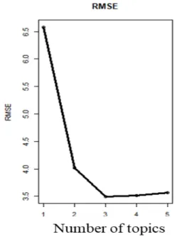
The number of topics needs to be fixed to construct covariate of features in social media and we use the criterion of root mean squared error (RMSE) of forecasts for test data to choose the number of topics. This measure is shown in Fig 4.2 when the number of topics changes from one to five. T suggests three topics for our social media.
Fig. 4.2 Evaluating Number of Topics
LDTM lets us detect changes in each topic, implying potential changes in customer interest. The top words among topics appear in Table 4.1. We interpret the topics as fol-lows.
1. Topic 1 (Property-battery): because the frequent words are “nfc” (iPhone5), “apps,” “battery” (all), “face recognition,” and “fingerprint” (iPhone X).
2. Topic 2 (Comparison): because competitors and their product names appear contin-ually (s3, Samsung, Android) with the word “better.”
am).
4.3 Leading Property of Topics to Sales
Fig. 4.3 plots time series for sales and frequency (number of words) under three topics from 2012: Q4 to 2017: Q4. It shows that the frequency of each topic leads sales by one period.
Fig. 4.3 Time Series Plot of Sales and Topics
Table 4.2 shows cross-correlation of time lags of one and two periods with sales and frequency of three topics. They show all topics lead sales by one period with similar mag-nitudes of effect. There is no delayed relation after one period for Topics 1 and 2, although two lags could exist for Topic 3.
Table 4.1 Top Words within Each Topic
Table 4.2 Cross-correlation between Topics and Sales Table 4.3 Comparative Models
4.4 Model Comparison
We now compare 10 models by covariate, treatment of generation-specific heterogeneity of parameters, and hierarchical structure of parameters connecting current and previous generations (Table 4.3).
Models 1–4.
Model 1 observes the formula in Norton-Bass (1987). Model 2 mirrors Jiang and Jain (2012). Models 3 and 4 include topic variables. All models lack the structure to
connect generations except as an innovator parameter (i.e., no trans-generational
memory). Thus we call them 0th-order models.
Model 5 ~ Model 8.
Models 5–8 are structured for parameter shifts to the next generation as hierarchical models. Models 5 and 7 use only parameters of previous generations. Models 6 and 8 include additional variables for topics in their hierarchical models. These models can pre-dict one step ahead for a new product even before launch. These are first-order models.
Model 9 ~ Model 10.
Models 9 and 10 also are first-order models. The difference from Models 5–8 is the homogeneous coefficients of marketing mix variables between generations. To improve model performance, all previous studies including marketing mix assume that it is heter-ogeneous. We assume marketing variables are homogeneous for all generations to achieve parsimony.
We compare the 10 models in three measures: log of marginal likelihood (LMD), de-viance information criteria (DIC), and RMSEs of forecasts for training data (G1–G5) and test data (G6). We confirmed convergence for all models via Geweke’s test (Geweke, 1992) at 95% significance in Table 4.4.
Table 4.4 Model Evaluations
0th-order models (Models 1–4) cannot forecast sales of G6 as test data because they
lack structure to accommodate the shift of
(
m qG, G)
. Then we evaluate all first-order models by RMSE(Train), log of marginal likelihood and DIC, and RMSE (Test).Model 3 exhibits the best in-sample performance indicated by RMSE and log of mar-ginal likelihood. Accompanying the marketing mix with social media information sharp-ens forecasting precision. RMSE of the holdout sample and DIC suggest Model 10 has the best performance. This finding shows the effectiveness of topic models. Also, our assumption of a homogeneous marketing mix yields better fit to the holdout sample, in-dicating heterogeneity may lead models to over-fit training data.
Comparing models among the first-order group shows that those with topic variables (Models 6, 8, and 10) out-perform those without topics (Models 5, 7, and 9). In general, model fit erodes for models with more restrictions, but even in the training data RMSE and LMD of first-order models approach those of Model 3 (best among the zero-order group). First-order Models 6 and 10 exhibit larger LMD and smaller DIC than Model 3. This finding implies hierarchical models enhance model fit.
After examining RMSE of test data and DIC criteria, we chose Model 10 and examine the results of estimation and forecasting. Model 10 features no price effect. That is con-sistent with iPhones having higher prices across generations than competing mobile phones and with adopters of iPhones showing themselves insensitive to price.
4.5 Parameter Estimates
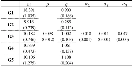
Parameter estimates of Model 10 are in Table 4.5, where number indicates posterior means and the posterior standard deviation is in parentheses.
Columns 𝑚𝑚 and show that estimates of 𝑚𝑚𝐺𝐺, 𝑞𝑞𝐺𝐺, and p are constant across generations. Coefficients α =i,i 1, 2, 3, are homogeneous among generations in response to covariates for Model 10.
Values of 𝑚𝑚𝐺𝐺, p, and 𝑞𝑞𝐺𝐺 define the curve for the G-th generation’s diffusion, and it is influenced by the topic feature of log
(
TopicGi(t−1) TopicGi(0))
.Estimates of 𝑚𝑚𝐺𝐺 imply that the market for G1 is potentially double that of other gener-ations. The first generation faces its original potential market. After the G2 launches, the market divides into an original and an influenced segment. As a result, its market is smaller than for the market for G1.
Estimates for imitation parameter 𝑞𝑞𝐺𝐺 increase slowly across all generations except G2. This finding suggests that consumers become imitators rather than innovators as genera-tions proceed and await reviews before buying new-generation products.
Quasi-t values (posterior mean divided by standard deviation) are large for
, 1, 2, 3
i i
α = , implying that all three topics are significant in this model. Topic
1(Property-battery) has expected negative correlations with sales. Topics 2(Competitor) and 3 (Dis-cussion) have significant positive correlations with sales.
Table 4.6 examines the hierarchical model’s estimates in Eq. (4.5).
Table 4.6 Estimates of Hierarchical Structure
We summarize results from Table 4.6 as follows.
(1) Estimated coefficients of 𝑚𝑚𝐺𝐺−1 and 𝑞𝑞𝐺𝐺−1 are nearly 1, indicating parameters for mar-ket size and imitation rate shift smoothly from previous generations. Estimates of 𝑚𝑚𝐺𝐺 decline gradually and estimates for 𝑞𝑞𝐺𝐺 increase across generations, expecting that
𝑚𝑚𝐺𝐺 declines because fewer new customers remain as the market matured and sales
were more influenced by previous generations and their marketing. After several gen-erations, 𝑞𝑞𝐺𝐺 trends upward with the popularity of products.
(2) We interpret the indirect topic effect from the estimated hierarchical structure as fol-lows. Topic 1(Property-battery) has significant positive correlations with 𝑚𝑚𝐺𝐺 and 𝑞𝑞𝐺𝐺. This finding implies that market size and imitation rate swell as consumers talked more about the property(battery) before launch. Topic 2 (Competitor) has a negative correlation with 𝑚𝑚𝐺𝐺 and a positive correlation on 𝑞𝑞𝐺𝐺. These findings mean that more communication on competitors attract imitators, but the risk to declining market size remains. Topic 3 (Discussion) has the effect opposite that of Topic 2.
(3) Indirect effects of topics in hierarchical models differ from direct effects in the adop-tion rate funcadop-tion as marketing mix variables. This finding implies different roles for social media pre- and post-launch. For instance, Topic 1(Property-battery) has a pos-itive indirect effect on parameter changes in the hierarchical structure and a negative direct effect on adoption rate function. These findings show that customers who were interested in properties of new generations before launch may be disappointed with them post-launch.
4.6 Forecasting Sales of Unlaunched New Generation
Using the estimated hierarchical structure and diffusion model parameter estimates, we can forecast sales of new generations before launch. Fig 4.4 shows forecast (solid line) of new-generation G6 and its actual sales (dashed line) during 2017Q4 to 2018Q3. Forecasts are accurate even if products were launched without using social media and prior structure on the parameter shifts inferred from hierarchical model.
Fig. 4.4 Forecasting Sales of Unlaunched New-Generation Products
5. Influence of Social Media on the Battery Problem
5.1 What is the battery problem?
Since early November of 2016, increasing numbers of iPhone 6 owners worldwide have complained their phones shut down unexpectedly even when adequately charged. Apple admitted that some phones needed their batteries replaced and offered to replace them gratis. In late 2016, Apple noted that some phones shut down "under normal conditions in order for the iPhone to protect its electronics." Although Apple tried to solve the battery problem by updating the iPhone OS, consumers complained on social media that their devices slowed after updating the OS. This problem caused by the battery appeared prom-inently on social media until late 2017. We focus on how social media discussion of the battery problem affected sales, leapfrogging, and switching of iPhones to subsequent gen-erations and competing products.
5.2 Acceleration Effect of Social Media on Leapfrogging to Competitor
Multi-generational diffusion models demonstrate the leapfrog effect, but discussions of it differ in the literature. Without mentioning leapfrog or switch effects explicitly, Norton and Bass (1987) distinguish independent from influenced markets. The former is the orig-inal or incremental market for current-generation products. The latter implies sales effects from previous generations.
Mahajan and Muller (1996) extend the Norton and Bass (1987) model to incorporate leapfrog and switch parameters into multi-generational diffusion of durable technological innovations. Jiang and Jain (2012) enlarge the model to consider how marketing mix
shapes diffusion of each generation where leapfrog and switch effects are incorporated as in the Norton-Bass model.
The blue line in the left panel of Fig 5.1 shows iPhone sales. It is hard from this figure to identify the influence of social media on the battery problem. Thus, we collect data for sales and market share of competing Android smartphones. Sales of Androids and total units, (iPhone plus Android) appear on the left and market shares on the right in Fig 5.1.
Fig. 5.1 Smartphone Unit Shares and Marketing Share
We seek to detect leapfrogging to a later iPhone generation and switching to Android smartphones induced by social media. Following Jiang and Jain (2012), we calculate them as
2( ) 1 1( ) 2( 2)
L t =m f t F t−τ (5.1)
2( ) 1 1( ) 2( 2)
S t =m F t f t−τ . (5.2) 𝐿𝐿2(𝑡𝑡) and 𝑆𝑆2(𝑡𝑡) are leapfroggers and switchers, respectively, from the first to the second
generation. L t is affected by the remaining fraction of first generation, and 2( ) S t is 2( ) affected by the installed fraction of first generation. The model detects switching from a previous to a later generation and leapfrogging after generations but not leapfrogging from iPhones to Androids. We then discuss how social media affect leapfrogging to a competitor using additional Android sales data.
Denote MS t as the market share of iPhones and q( ) TS t( ) as total unit sales of iPhones
and Androids at time t. Then we define
[
]
( ) ( ) G( ) G( 1) 2,
where D t( ) indicates the change in unit sales of iPhones corresponding to the total smartphone market. If we define SL t( ) as total leapfrogging from one iPhone to its later generation in period t, we derive the leapfrog effect from competitor CL t( ) by
( ) ( ) ( )
CL t =D t −SL t . (5.4)
We compare two kinds of leapfrogging from iPhones and Androids via the ratio ( ) ( ) ( ) SL t rate t CL t =
.
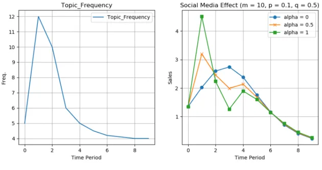
(5.5)From 2016:Q4 through 2017:Q4, the period of the battery problem, iPhone unit sales did not decrease significantly (left of Fig. 5.1), but the market share of iPhones declined during the two preceding years. To detect how social media coverage of the battery prob-lem affected sales, we compare two models—one including topics extracted from social media and one that ignores them. Fig. 5.2 shows a numerical example of the social media effect when one topic is included in the model.
Fig. 5.2 Social Media Effect
The left panel of Fig. 5.2 shows topic frequency. It implies the influence on sales by comparing the model that estimated 𝛼𝛼𝐺𝐺 and that which estimated 𝛼𝛼𝐺𝐺 = 0. The “alpha” in the right panel of Fig. 5.2 depicts sales corresponding to three kinds of value, (𝛼𝛼𝐺𝐺=0, 0.5, 1) when we fix the parameters as (m=10, p=0.1, q=0.5). 𝛼𝛼𝐺𝐺 = 0 indicates the model with-out social media effects. Social media become more influential as 𝛼𝛼𝐺𝐺 increases.
Fig. 5.3 reveals leapfrogging (SL t( )) among iPhone generations with and without the
social media effect. Social media exert greater influence for later generations, implying that consumers were more influenced as generations proceeded.
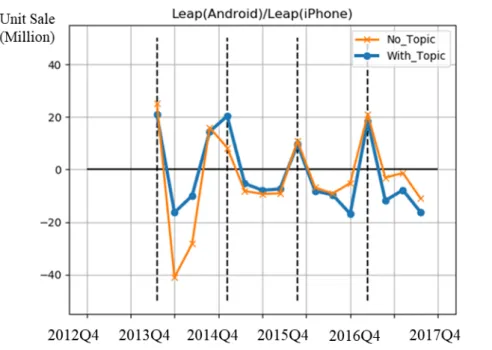
Fig 5.4 plots 𝑟𝑟𝑟𝑟𝑡𝑡𝑟𝑟(𝑡𝑡) from Eq. (5.5). A negative value means more customers leap-frogged to iPhones than to Androids. A positive value means more leapleap-frogged to An-droids. To evaluate SL t( ) in the model lacking social media effects, we enforced 0 as the value of 𝜶𝜶𝑮𝑮. Then we measured the effect of social media by the difference between these two leapfrogs estimates (Fig. 5.5).
Fig. 5.3 Leapfrog Effect of iPhone
Fig. 5.4 Comparison of Leapfrogging between iPhone and Android
Fig. 5.5 Difference in Leapfrogging
In Fig 5.5, over periods with positive unit sales, which implies social media were sig-nificant with respect to the battery problem, unit sales of iPhones decline gradually. Peri-ods with negative sales mean social media had a negative effect on iPhones. Starting with iPhone 5, the social media effect slowly erodes unit sales of iPhones. When the battery problem was exposed in 2016:Q4, the social media effect was distinguished by leapfrog-ging to Android. Social media had a significant influence on product diffusion.
6. Conclusion
This study proposed a multi-generational diffusion model with social media effects that included a hierarchical structure connecting diffusion parameters of successive genera-tions. Results show the effects of social media using a dynamic labeled topic model di-rectly on the adoption rate function as effective marketing mix as well as indidi-rectly on
the parameter change described by hierarchical model on the shift of diffusion parameters to next generation.
Unlike previous multi-generational diffusion models, ours forecasts sales of new-gen-eration products before launch using social media as the leading indicator and the hierar-chical model.
Finally, our model featuring social media effects improves the precision of forecasting and shows how social media affected sales of smartphones via leapfrogging and switching to next-generation and competing products. We examined how iPhone’s battery problem affected sales, leapfrogging, and switching to later-generation iPhones and competing Androids.
Further issues remain. We proposed the LDTM to extract dynamic features hidden in social media and confirmed that “people chat before they act.” However, results of the model depend on prior LDTM settings. Determining the full robustness of dynamic text analysis awaits future studies.
References
1. Ansari, A., Li, Y. and Zhang, J.Z. (2018), “Probabilistic Topic Model for Hybrid Rec-ommender Systems: A Stochastic Variational Bayesian Approach,” Marketing Science, 37(6), 987-1008.
2. Bass, F.M. (1969), “A New Product Growth for Model Consumer Durables,”
Manage-ment Science, 15(5), 215-227.
3. Bass, F.M. (1980), “The Relationship between Diffusion Rates, Experience Curves, and Demand Elasticities for Consumer Durable Technological Innovations,” The
Jour-nal of Business, 53(3), 51-67.
4. Bass, F.M., Krishnan T.V and Jain D.C (1994), “Why the Bass Model Fits without De-cision Variables,” Marketing Science, 13(3), 203-326.
5. Bewley, R. and Fiebig, D. (1988), “Estimation of Price Elasticities for an International Telephone Demand Model,” Journal of Industrial Economics, 36(4), 393-409.
6. Blei, D.M., Ng A.Y. and Jordan, M.I. (2003) “Latent Dirichlet Allocation,” Journal of
Machine Learning Research, 3, 993-1022.
7. Blei D.M. and Lafferty J.D (2006), “Dynamic Topic Model,” ICML '06 Proceedings of
the 23rd international conference on Machine learning, 113-120.
8. Danaher, P.J., Hardie, B.G.S. and Putsis, W.P. (2001), “Marketing-Mix Variables and the Diffusion of Successive Generations of a Technological Innovation,” Journal of
Marketing Research, 38(4), 501-514.
9. Daniel R., Daniel H., Ramesh N., Christopher D.M. (2009), “Labeled LDA: A Super-vised Topic Model for Credit Attribution in Multi-Labeled Corpora,” Proceedings of
the 2009 Conference on Empirical Methods in Natural Language Processing, 248-256.
10. Eastingwood, C.J., Mahajan, V. and Muller, E. (1983), “A Nonuniform Influence Inno-vation Diffusion Model of New Product Acceptance,” Marketing Science, 2(3), 203-317.
11. Geweke, J. (1992). “Evaluating the accuracy of sampling‐based approaches to the cal-culation of posterior moments,” In Bayesian Statistics 4, Bernardo, J.M., Berger, J. O., Dawid, A.P. and Smith, A.F.M. (eds.), 169‐193. Oxford: Oxford University.
12. Griffiths T.L., Steyvers M. and Tenenbaum J.B. (2007), “Topics in Semantic Represen-tation,” Pychology Reviews, 114(2), 211-244.
13. Guo, Z.L. and Chen, J.Q. (2018), “Multi-Generation Product Diffusion in the Presence of Strategic Consumers,” Information Systems Research, 29(1), 206-224.
14. Hosrky, D. and Simon, L.S. (1983), “Advertising and the Diffusion of New Products,”
15. Horsky, D. (1990), “A Diffusion Model Incorporating Product Benefits, Price, Income and Information,” Marketing Science, 9(4), 279-365.
16. Hruschka, H. (2015) “Linking Multi-Category Purchases to Latent Activities of Shop-pers: Analyzing Market Baskets by Topic Models,” University of Regensburg Working
Papers in Business, Economics and Management Information Systems, 482, 1-3.
17. Jiang, Z.R. (2010), “How to Give Away Software with Successive Versions,” Decision
Support Systems, 49(4), 430-441.
18. Jiang Z.R. and Jain D.C (2012), “A Generalized Norton–Bass Model for Multigenera-tion Diffusion,” Management Science, 58(10), 1887-1897.
19. Jun, D.B. and Park Y.S. (1999) “A choice-based diffusion model for multiple genera-tions of products,” Technology Forecasting and Social Change, 61(1), 45-58.
20. Kim, N. Chang, D. and Shoker, A. (2000), “Modeling Intercategory Dynamics for a Growing Information Technology Industry,” Management Science, 46(4), 496-512. 21. Li, Y. and Terui, N. (2018) “Social Media and the Diffusion of an Information
Tech-nology Product,” J. Chen et al.(Eds.) Knowledge and Systems Sciences, vol.949, 171-185, Springer.
22. Mahajan, V. and Muller, E. (1981), “A Nonsymmetric Responding Logistic Model for Forecasting Technological Substitution,” Technology Forecasting and Social Change, 21(3), 199-213.
23. Mahajan, V. and Muller, E. (1996), “Timing, Diffusion, and Substitution of Successive Generations of Technological Innovations: The IBM Mainframe Case,” Technological
Forecasting and Social Change, 51(2), 213-224.
24. Netzer, O., Feldman, R., Goldenberg, J. and Fresko, M. (2012), Mine Your Own Busi-ness: Market-Structure Surveillance Through Text Mining,” Marketing Science, 31 (3), 521-543.
25. Norton, J.A. and Bass, F.M. (1987), “A Diffusion Theory Model of Adoption and Sub-stitution for Successive Generations of High-Technology Products,” Management
Sci-ence, 33(9), 1069-1086.
26. Robinson B. and Lakhani C. (1975), “Dynamic Price Models for New-Product Plan-ning,” Management Science, 21(10), 1089-1214.
27. Speece, M. and MacLachlan, D.L. (1995), “Application of a Multi-Generation Diffu-sion Model to Milk Container Technology,” Technological Forecasting and Social
Change, 49(3), 281-295.
28. Terui, N., Ban, M. and Maki, T. (2010), “Finding Market Structure by Sales Count Dy-namics - Multivariate Structural Time Series Models with Hierarchical Structure for Count Data,“ Annals of the Institute of Statistical Mathematics, 62, 92-107.
29. Terui, N. and Ban, M. (2014), “Multivariate Structural Time Series Models with Hier-archical Structure for Over-dispersed Discrete Outcome,” Journal of Forecasting, 33, 376-390.
30. Tirunillai, S. and Tellis, G.J. (2014), “Mining marketing meaning from online chatter: Strategic brand analysis of big data using latent dirichlet allocation,” Journal of
Mar-keting Research, 51(4), pp. 463-479.
31. Von Bertalanffy, L. (1957), “Quantitative Laws in Metabolism and Growth,” The
Appendix.
A. Labeled Dynamic Topic model
The DTM is base model for LDTM as detailed in Blei and Lafferty (2006). Based on DTM, we assume the word “battery” belongs to Topic 1 in this study. The algorithm of LDTM can be written as For t = 1,2, …, T 1. Draw Topics 𝛽𝛽𝑏𝑏,𝑘𝑘�𝛽𝛽𝑏𝑏−1,𝑘𝑘 ~ 𝛮𝛮�𝛽𝛽𝑏𝑏−1,𝑘𝑘, 𝜎𝜎2𝐼𝐼� 2. Draw at 𝛼𝛼𝑏𝑏|𝛼𝛼𝑏𝑏−1 ~ 𝛮𝛮(𝛼𝛼𝑏𝑏−1, 𝛿𝛿2𝐼𝐼)
For each document: 3. Topic proportion 𝜂𝜂𝐺𝐺,𝑑𝑑|𝛼𝛼𝑏𝑏 ~ 𝑁𝑁(𝛼𝛼, 𝑟𝑟2𝐈𝐈)
𝜃𝜃𝐺𝐺,𝑑𝑑|𝜂𝜂𝐺𝐺,𝑑𝑑~ 𝜋𝜋�𝜂𝜂𝐺𝐺,𝑑𝑑� For each word:
if word == ‘battery’: 𝑧𝑧𝑏𝑏,𝑑𝑑,𝑛𝑛 = 1 else: 4. Topic-word assignment 𝑧𝑧𝑏𝑏,𝑑𝑑,𝑛𝑛|𝜃𝜃𝑏𝑏,𝑑𝑑 ~ 𝑀𝑀𝑀𝑀𝑀𝑀𝑡𝑡𝑇𝑇𝑀𝑀𝑇𝑇𝑚𝑚𝑇𝑇𝑟𝑟𝑀𝑀�𝜃𝜃𝑏𝑏,𝑑𝑑� 𝑤𝑤𝑑𝑑,𝑛𝑛|𝑧𝑧𝑑𝑑,𝑛𝑛�𝛽𝛽𝑏𝑏,𝑘𝑘� ~ 𝑀𝑀𝑀𝑀𝑀𝑀𝑡𝑡𝑇𝑇𝑀𝑀𝑇𝑇𝑚𝑚𝑇𝑇𝑟𝑟𝑀𝑀 �𝜋𝜋�𝛽𝛽𝑏𝑏,𝑧𝑧𝑑𝑑,𝑧𝑧��
B. MCMC method for the Bass model B.1 Prior Settings for the Bass model
Parameter Setting 𝑚𝑚𝐺𝐺 ~ 𝑁𝑁(𝜇𝜇𝑚𝑚0, 𝜏𝜏𝑚𝑚0−1) 𝜇𝜇𝑚𝑚0 = 0, 𝜏𝜏𝑚𝑚0 = 0.1 𝑞𝑞𝐺𝐺 ~ 𝑁𝑁�𝜇𝜇𝑞𝑞0, 𝜏𝜏𝑞𝑞0−1� 𝜇𝜇𝑞𝑞0 = 0, 𝜏𝜏𝑞𝑞0= 0.1 𝑝𝑝 ~ 𝑁𝑁�𝜇𝜇𝑝𝑝0, 𝜏𝜏𝑝𝑝0−1� 𝜇𝜇𝑝𝑝0 = 0, 𝜏𝜏𝑝𝑝0 = 0.1 𝑋𝑋𝐺𝐺 ~ 𝑁𝑁(𝜇𝜇𝑋𝑋, 𝜏𝜏𝑋𝑋−1) 𝜇𝜇𝑋𝑋0 = 0, 𝜏𝜏𝑋𝑋0 = 0.1 σ~ 𝐼𝐼𝐼𝐼(𝑟𝑟, 𝑏𝑏) a = 3, b = 10 𝛼𝛼𝐺𝐺 ~ 𝑁𝑁(𝜇𝜇α0, 𝜏𝜏α0−1) 𝜇𝜇𝛼𝛼0= 0, 𝜏𝜏α0= 0.1 𝜷𝜷𝑮𝑮 ~ 𝑁𝑁�𝜇𝜇β0, 𝜏𝜏β0−1� 𝜇𝜇𝛽𝛽0= 0, 𝜏𝜏β0 = 0.1 σ𝑥𝑥~ 𝐼𝐼𝐼𝐼(𝑟𝑟, 𝑏𝑏) a= 3, b = 10 Θ~ 𝑁𝑁(𝜇𝜇Θ0, 𝜏𝜏Θ0−1) 𝜇𝜇Θ0= 0, 𝜏𝜏Θ0= 0.1 𝚵𝚵~ 𝐼𝐼𝐼𝐼(𝑟𝑟, 𝑏𝑏) a = 3, b = 10
* 𝛅𝛅 is the vector of �Δ𝑚𝑚, Δ𝑞𝑞, 𝜎𝜎𝛼𝛼, 𝜎𝜎𝛽𝛽�, 𝚵𝚵 is the vector of �𝜎𝜎𝑚𝑚, 𝜎𝜎𝑞𝑞, 𝜎𝜎𝛼𝛼, 𝜎𝜎𝛽𝛽�. B.2 Conditional Posterior Distributions
(1)
For iter (=1, …, R) of MCMC iterations, we use Metropolis-Hastings with a random walk algorithm for each generation G,
𝑚𝑚𝐺𝐺(𝐺𝐺𝑏𝑏𝑏𝑏𝑏𝑏)= 𝑚𝑚𝐺𝐺(𝐺𝐺𝑏𝑏𝑏𝑏𝑏𝑏−1)+ 𝜆𝜆𝑚𝑚; 𝜆𝜆𝑚𝑚 ~ 𝑁𝑁(0,0.05), (B. 1)
where the acceptance probability is
α = min �1, 𝑝𝑝�𝑚𝑚𝐺𝐺 (𝐺𝐺𝑏𝑏𝑏𝑏𝑏𝑏) | {𝑦𝑦 𝐺𝐺, 𝑡𝑡, 𝑋𝑋𝐺𝐺}, {𝑝𝑝, 𝑞𝑞𝐺𝐺}, 𝜎𝜎� 𝑝𝑝�𝑚𝑚𝐺𝐺(𝐺𝐺𝑏𝑏𝑏𝑏𝑏𝑏−1) | {𝑦𝑦𝐺𝐺, 𝑡𝑡, 𝑋𝑋𝐺𝐺}, {𝑝𝑝, 𝑞𝑞𝐺𝐺}, 𝜎𝜎� � , (B. 2) where t = 1, …, N and G = 1, 2, …, 5. | { , , }{ , }, G G G G m y t X p q σ
(2)
For pand 𝑞𝑞𝐺𝐺, we also use Metropolis-Hastings sampling, which is the same as 𝑚𝑚𝐺𝐺 above.
. (B.3) The probability of acceptance is
min �1, 𝑝𝑝�𝑝𝑝 (𝐺𝐺𝑏𝑏𝑏𝑏𝑏𝑏) | {𝑦𝑦 𝐺𝐺, 𝑡𝑡, 𝑋𝑋𝐺𝐺}, {𝑚𝑚𝐺𝐺, 𝑞𝑞𝐺𝐺}, 𝜎𝜎� 𝑝𝑝�𝑝𝑝(𝐺𝐺𝑏𝑏𝑏𝑏𝑏𝑏−1) | {𝑦𝑦𝐺𝐺, 𝑡𝑡, 𝑋𝑋𝐺𝐺}, {𝑚𝑚𝐺𝐺, 𝑞𝑞𝐺𝐺}, 𝜎𝜎� � . (B. 4) (3) 𝑞𝑞𝐺𝐺(𝐺𝐺𝑏𝑏𝑏𝑏𝑏𝑏)= 𝑞𝑞𝐺𝐺(𝐺𝐺𝑏𝑏𝑏𝑏𝑏𝑏−1)+ 𝜆𝜆𝑞𝑞; 𝜆𝜆𝑞𝑞 ~ 𝑁𝑁(0,0.05). (B.5)
The acceptation probability is
min �1, 𝑝𝑝�𝑞𝑞𝐺𝐺 (𝐺𝐺𝑏𝑏𝑏𝑏𝑏𝑏) | {𝑦𝑦 𝐺𝐺, 𝑡𝑡, 𝑋𝑋𝐺𝐺}, {𝑚𝑚𝐺𝐺, 𝑝𝑝}, 𝜎𝜎� 𝑝𝑝�𝑞𝑞𝐺𝐺(𝐺𝐺𝑏𝑏𝑏𝑏𝑏𝑏−1) | {𝑦𝑦𝐺𝐺, 𝑡𝑡, 𝑋𝑋𝐺𝐺}, {𝑚𝑚𝐺𝐺, 𝑝𝑝}, 𝜎𝜎� � . (B. 6) (4) 𝑋𝑋𝐺𝐺(𝐺𝐺𝑏𝑏𝑏𝑏𝑏𝑏) = 𝑋𝑋𝐺𝐺(𝐺𝐺𝑏𝑏𝑏𝑏𝑏𝑏−1)+ 𝜆𝜆𝑋𝑋; 𝜆𝜆𝑋𝑋 ~ 𝑁𝑁(0,0.05). (B. 7)
The acceptation probability is
min �1, 𝑝𝑝�𝑋𝑋𝐺𝐺 (𝐺𝐺𝑏𝑏𝑏𝑏𝑏𝑏) | {𝑦𝑦 𝐺𝐺, 𝑡𝑡, }, {𝑚𝑚𝐺𝐺, 𝑞𝑞𝐺𝐺, 𝑝𝑝}, 𝜎𝜎� 𝑝𝑝�𝑋𝑋𝐺𝐺(𝐺𝐺𝑏𝑏𝑏𝑏𝑏𝑏−1) | {𝑦𝑦𝐺𝐺, 𝑡𝑡}, {𝑚𝑚𝐺𝐺, 𝑞𝑞𝐺𝐺, 𝑝𝑝}, 𝜎𝜎� � . (B. 8) (5) σ | {𝑦𝑦𝐺𝐺, 𝑡𝑡, 𝑿𝑿𝑮𝑮}, {𝑚𝑚𝐺𝐺, 𝑞𝑞𝐺𝐺, 𝑝𝑝}
If we define estimated sales in period t for the Gth generation as
y�𝐺𝐺𝑏𝑏 = 𝑓𝑓({𝑦𝑦𝐺𝐺, 𝑡𝑡, 𝑋𝑋𝐺𝐺}, {𝑚𝑚𝐺𝐺, 𝑞𝑞𝐺𝐺}), (B. 9)
we can update σ by
𝐼𝐼𝐼𝐼 �a +2 , b +n ∑ (y𝑛𝑛𝑏𝑏=1 𝑏𝑏− ∑2 𝑀𝑀𝐺𝐺=1y�𝐺𝐺𝑏𝑏)2� , (B. 10)
M stands for number of generations in this equation.
| { G, , G}{ G, G}, p y t X m q σ ( ) ( 1)
(
)
;
0, 0.05
iter iter p pp
=
p
−+
λ λ
N
| { , , }{ , }, G G G G q y t X m p σ | { , }{ , , }, G G G G X y t m q p σMarketing Mix.
(6)
For each topic j the posterior of coefficient 𝛼𝛼𝐺𝐺𝐺𝐺can be derived from a normal regression equation from 𝑁𝑁 �(𝑀𝑀σ𝛼𝛼+ σ𝛼𝛼0)−1�σ𝛼𝛼� �𝑋𝑋𝐼𝐼𝑇𝑇 − 𝑽𝑽𝑮𝑮𝐺𝐺∙ 𝛽𝛽𝐺𝐺− � 𝑇𝑇𝑇𝑇𝑝𝑝𝑇𝑇𝑇𝑇𝐺𝐺𝑘𝑘𝐺𝐺∙ 𝛼𝛼𝐺𝐺𝑘𝑘 𝑇𝑇≠𝐺𝐺 𝑘𝑘=1 � 𝑇𝑇𝑇𝑇𝑝𝑝𝑇𝑇𝑇𝑇𝐺𝐺𝐺𝐺−1 𝑛𝑛 𝐺𝐺=1 + 𝜇𝜇𝛼𝛼0σ𝛼𝛼0� , (𝑀𝑀σ𝛼𝛼+ σ𝛼𝛼0)−1�
(
)
1(
)
1 ( ) ( ) ( ) ( ) G G G G G G G G G G G m f t τ F t τ y − t F t τ Y − t f t τ ≡ − − + − + − (𝐵𝐵. 11) (7) 𝑁𝑁 ��𝑀𝑀σ𝛽𝛽+ σ𝛽𝛽0�−1�σ𝛼𝛼�(𝑋𝑋𝐼𝐼𝑇𝑇 − 𝑻𝑻𝑻𝑻𝑻𝑻𝑻𝑻𝑻𝑻𝑮𝑮𝑻𝑻∙ 𝜶𝜶𝑮𝑮 )𝑉𝑉𝐺𝐺−1 𝑛𝑛 𝐺𝐺=1 + 𝜇𝜇𝛽𝛽0σ𝛽𝛽0� , �𝑀𝑀σ𝛽𝛽+ σ𝛽𝛽0�−1� (𝐵𝐵. 12) (8) 𝐼𝐼𝐼𝐼 �α +2 , β +n ∑ (X𝑛𝑛𝐺𝐺=1 𝐺𝐺𝐺𝐺− 𝑻𝑻𝑻𝑻𝑻𝑻𝑻𝑻𝑻𝑻2𝑮𝑮𝑻𝑻∙ 𝜶𝜶𝑮𝑮− 𝑽𝑽𝑮𝑮𝐺𝐺∙ 𝛽𝛽𝐺𝐺)2� . (B. 13) Hierarchical Structure. (9)Assuming D as data matrix for hierarchical structure, we can derive the posterior of co-efficient 𝛿𝛿𝑚𝑚𝐺𝐺 by 𝑁𝑁 �(𝑀𝑀σ𝑚𝑚+ σ𝑚𝑚0)−1�σ𝑚𝑚� �𝑚𝑚𝐼𝐼 − �(𝐷𝐷𝐺𝐺𝑧𝑧∙𝛿𝛿𝑚𝑚𝑧𝑧) 𝐾𝐾≠𝐺𝐺 𝑧𝑧=1 � 𝐷𝐷𝐺𝐺𝐺𝐺−1 𝑀𝑀 𝐺𝐺=1 + 𝜇𝜇𝑚𝑚0σ𝑚𝑚0� , (𝑀𝑀σ𝑚𝑚+ σ𝑚𝑚0)−1�. (B. 14)
{
}
| , , , , , G XG t G G α σx α LTopic V Δ{
}
G | XG, ,t G, G , , x β LTopic V Δβ σ{
G} {
}
| , , , , , x G XG t G G σ α β LTopic V{
1} { }
| m mG, G− , G ,σm m Δ T{
} { }
σ Δ𝐼𝐼𝐼𝐼 �α +n2 , β +∑ �m𝐺𝐺− ∑ (𝐷𝐷𝑧𝑧=1 𝐺𝐺𝑧𝑧∙𝛿𝛿𝑚𝑚𝑧𝑧)�
2 𝑀𝑀
𝐺𝐺=1
2 � . (B. 15)
As the sampling methods are the same among all the hierarchical structures, we can sample for other parameters (𝚫𝚫𝒒𝒒, 𝚫𝚫𝜶𝜶 𝑟𝑟𝑀𝑀𝑎𝑎 𝚫𝚫𝜷𝜷) as well.
Forecasting
(10)
For 𝑇𝑇𝑡𝑡𝑟𝑟𝑟𝑟 = 1, … , ITER, after sampling all the parameters using MCMC, the forecast-ing unit sales for the G-th generation 𝑦𝑦𝐺𝐺(𝑡𝑡) can be written as
(B.16) where
(
)
(
(
(
)
((
)(
( ))
()
))
)
( ) ( ) ( ) ( ) ( ) 1 exp ( ) ( ) ( ) 1+ exp ( ) | , =iter iter iter G G
iter iter iter iter iter
G G G G G p q X t iter iter q / p p q X t F t p q − − + − + . (B.17) Note that (B.18)
then total sales can be calculated by
( ) ( ) ( ) iter G( ) iter G y t =
∑
y t . (B.19) ( ) | G, G, , G( ), G, G( 1), G( ) y t m q p X t T LTopic t− V t(
)
(
)
( ) ( ) 1 1 1 2 ( ) ( ) 1 1 1 2 2 2 ( ) ( ) ( ) ( ) , , ( ) ( ) 1 , , ( ) ( ) iter iter iter iter iter iter G G G G G y t m f t t y t m f t F t t y t m f t F t τ τ τ τ = < = − − ≥ = −(
)
(
)
(
)
(
)
1 ( ) ( ) 1 1 ( ) ( ) 1 ( ) ( ) 1 1 , 1 , ( ) ( ) ( ), ( ) ( ( ) , 1 , ( ) ( ) ( G G G iter iter G G G G G G iter iter G G G G G G G iter iter G G G G G t G N y t F t Y t f t y t m f t F t t G N y t F t Y t f τ τ τ τ τ τ τ τ τ + − − + − − − ≤ < < ≤ + − + − = − − ≥ < ≤ + − +(
)
(
1 1)
)) 1 , G G G t τ F + t τ + − × − − (
)
( ) ( ) ( ) ( ) ( ) , ( ) log ( ) (0) ' ( 1), iter G Giter iter iter
G G G G G G G X t t t X t t V t V t t τ β τ = < = + + − ≥ α LTopic ( ) ( ) iter y t
Table 4.1 Cross-correlation between Topics and Sales
Table 4.2 Top Words of Each Topic
Topic 1 Topic 2 Topic 3
t -0.193 -0.271 -0.051
t-1 0.575 0.575 0.688
t-2 0.097 0.020 0.286
Topic 1 iPhone 5 iPhone 5s iPhone 6 iPhone 6s iPhone 7 iPhone X/8
1 apple apple phone apple apple apple
2 time battery apple battery ios face
3 new ios android ios phone phone 4 iphone use ios phone android id
5 market apps use time charging charging 6 device problem time back back recognition
7innovation phone apps charging battery fingerprint
8 nfc update problem new fast like 9 apples app device apps time screen 10 like like new jack wireless innovation
Topic 2 iPhone 5 iPhone 5s iPhone 6 iPhone 6s iPhone 7 iPhone X/8
1 iphone iphone iphone iphone iphone iphone
2 5 5s 6s 7 8 s8
3 samsung android 6 plus plus samsung
4 better better better better 7 x
5 galaxy samsung samsung ram x 8
6 4s s4 camera camera better display 7 s3 phone android samsung 5 screen
8 ios 5 ram screen s8 better
9 screen camera plus 6s screen android
10 lumia good s6 s7 display ram
Topic 3 iPhone 5 iPhone 5s iPhone 6 iPhone 6s iPhone 7 iPhone X/8
1 iPhone 5 iphone iphone iphone iphone iphone 2 apple phone phone phone phone phone 3 phone buy apple buy apple apple
4 iphone u dont apple dont x
5 dont dont buy dont buy dont
6 u 5s like like like buy
7 buy apple people u people like
8 like one best phones one want
9 people im one android im better
Property Comparison Discussion
𝜑
2,𝑣
𝑏𝑏
𝜑
1,𝑣
𝑏𝑏
𝜑
3,𝑣
𝑏𝑏
T ab le 4.3 C om p ar at ive M od el s
Table 4.4 Model Evaluations
Table 4.5 Parameter Estimates
Table 4.6 Estimates of Hierarchical Structure
Model 1 2 3 4 5 6 7 8 9 10 RMSE(Train) 3.251 3.215 2.883 3.059 4.217 3.766 3.649 3.038 3.587 2.897 RMSE(Test) - - - - 9.097 5.091 8.881 4.987 3.552 3.495 log(ml) -95.07 -90.57 -75.6 -75.9 -85.56 -74.48 -84.473 -75.993 -85.92 -75.911 DIC 258.4 250.5 207.18 208.88 269.52 211.57 271.43 205.55 241.58 196.1 Zeroth-Order First-Order m p q 18.391 0.900 (1.035) (0.186) 9.916 0.285 (0.739) (0.112) 10.182 1.002 (0.746) (0.103) 10.839 1.061 (0.473) (0.137) 10.106 1.108 (1.275) (0.204) G1 G2 G3 G4 G5 0.098 (0.012) -0.018 (0.001) 0.011 (0.001) 0.047 (0.000) 𝛼𝛼1 𝛼𝛼2 𝛼𝛼3 intercept 0.037 0.031 -0.025 0.022 0.976 (0.002) (0.002) (0.001) (0.001) (0.001) -0.014 0.036 0.011 -0.049 1.010 (0.000) (0.001) (0.002) (0.001) (0.001) 𝛿𝛿𝑚𝑚 𝛿𝛿𝑞𝑞 𝑇𝑇1 𝑇𝑇2 𝑇𝑇3 𝑚𝑚(𝑞𝑞)𝐺𝐺−1
Fig. 3.1 Role of Social Media before and after Launch
Fig. 4.4 Forecasting Sales of Unlaunched New Generation
Fig. 5.4 Leapfrog Effect Comparison between iPhone and Android