著者
NAKAMORI Seiichi, YAMAMOTO Naoki
journal or
publication title
Bulletin of the Faculty of Education,
Kagoshima University. Natural science
volume
62
page range
43-63
A New Face Recognition Method
Using QR Decomposition
NAKAMORI Seiichi* and YAMAMOTO Naoki** (Received 26 October, 2010)
Abstract
This paper presents a new face recognition method using the QR decomposition. The face recognition method is compared with the face recognition method by the snapshot Principal Component Analysis (PCA) mainly from the viewpoint of the computation time consumed for the face recognition. The recognition is based on the distance, measured by the L2 norm, between the vector of the projected test face image and the vectors of the projected training face images. Specifically, each image is stored in a vector of size
N N. Instead of an N x N covariance matrix in the PCA, as in the snapshot PCA method, Eigenspace is created from a P x P covariance matrix, where P is the number of persons or training images.
Some pattern recognition examples are shown, It is found that the proposed snapshot QR decomposition method is preferable, in face recognition, to the snapshot PCA method.
Keyword : Principal Component Analysis, Face recognition, QR decomposition, Pattern recognition, Snapshot PCA method
* Professor of Kagoshima University , Faculty of Education ** Part-time lecturer
The Principal Component Analysis (PCA) is one of the most successful techniques
that have been applied to feature extraction, data compression, pattern recognition and
face recognition, etc. The PCA is known as a statistical method with a relation to factor
analysis. The face recognition can be categorized into face identification, face
classification, or sex determination. The most useful applications contain crowd
surveillance, video content indexing, personal identification (e.g. driver's license), mug
shots matching and entrance security, etc. The main idea of using the PCA for face
recognition is to express the large one-dimensional vector of pixels constructed from
two-dimensional face image into the compact principal components of the feature space
[1], [2]. This can be called eigenspace projection. Eigenspace is calculated by identifying
the eigenvectors of the covariance matrix derived from a set of face images (vectors).
The method outlined above can lead to extremely large covariance matrices. For
example, images of size 112 x 92 combine to create a data matrix of size N x P,
N =10304 , where P is number of persons or training images to be recognized, and a
covariance matrix of size 10304 x10304 must be used in the calculation for the face
recognition. This is a problem because calculating the covariance matrix and the
eigenvectors/eigenvalues of the covariance is computationally demanding. Instead of
the PCA, in the snapshot PCA, a P x P covariance matrix is used to create the
eigenspace rather than a 10304 x 10304 covariance matrix.
This paper presents a new face recognition method using the QR decomposition. For
the variance matrix Si, of (1) in [3], the QR decomposition is applied as
In the current method, the P x P covariance matrix
in the snapshot PCA is
factorized by the QR decomposition. Specifically, each training image is stored in a
vector of size N. Instead of the N x N covariance matrix, as in the snapshot PCA
method, eigenspace is created from the P x P covariance matrix, where P is the
number of persons or training images. Each of the mean centered vectors ( ) of the
training images is projected into the eigenspace. The projection of the mean centered
training images into the eigenspace is calculated by (14). Each test image is first mean
centered by subtracting the mean image, and is then projected into the same eigenspace
defined by Q. The vector of the projected test image is compared with every vector of
the projected training image. The vector of the projected training image, that is the
closest to the vector of the projected test image, based on the distance measure, is
recognized as the most similar image to the test image. In this paper, as the similarity measure, the L_2 norm is used.
The proposed snapshot QR decomposition method for the face recognition is compared with the snapshot PCA method mainly from the point of the computation time
consumed for recognizing the test face image, based on the values of the L_2 norm, between the vector of the projected test face image and the vectors of the projected training face images.
In section 2, at first, the PCA is introduced. Then, the snapshot PCA method is explained from the viewpoint of computer storage memory. Finally, the snapshot recognition method, based on the QR decomposition, is proposed. In Section 3, to compare the proposed snapshot QR decomposition method with the snapshot PCA method, three pattern recognition examples are shown
2. Pattern recognition methods
2.1 Image recognition by Principal Component Analysis (PCA) [2]
In this section, Principal Component Analysis [2] is introduced, since the PCA is a
fundamental technique in pattern recognition. The PCA is implemented, according to the
following steps.
Step (1)
Let each image be stored in an N x l column vector as
Here, P denotes the number of persons or training images. Let m be the mean vector of the P number of persons or training image vectors x^1, x^2, • • •x^P .
Let represent the mean centered image vectors, which are calculated by subtracting the mean vector m from the training image vectors x^i as
Step (2)
Step (3)
Let be the covariance matrix given by
Step (4)
Let V consist of eigenvectors corresponding to eigenvalues, which are the diagonal elements of a matrix .
Let us introduce an N x P matrix V , where the eigenvectors v_i V , corresponding to non-zero eigenvalues , are ordered from their large to small values, e.g.
Step (5)
Let us project each of the mean centered training vectors , i = 1, 2, • • •, P, into the eigenspace V. This projection is calculated by the dot product of the mean centered training images with each of the ordered eigenvectors.
Henceforth, the dot product of the mean centered training images and the first eigenvectors generates the first component values in the vectors .
Step (6)
Let be an N x l vector, which corresponds to the test image. Let be the mean centered vector obtained by subtracting the mean vector m of the training image vectors from .
Let us project the vector into the eigenspace given by as
The projected test vector is compared with the projected training vectors , i =1, 2, • • • P. respectively. The test image with the closest measure to the training image is found to be the face of the most similar person of the training images, and the unknown test image is identified. In this paper, as similarity between the training images and the test image, the measure by the L_2 norm is used.
However, the PCA method, described above, leads to the covariance matrices with extremely large dimensions. For example, for the 112 x 92 dimensional matrix of the training image, the dimensions of the matrix of (4) become 10304 x P P. The size of the covariance matrix of (5) is 10304 x 10304 . In the PCA method, the calculation of the covariance matrix might be difficult, because, due to the limited main memory, it is impossible for the personal computer to storage all the matrix elements of the covariance matrix. Hence, the face recognition, based on the PCA, could not be proceeded to the next step of calculating the eigenvalues and the eigenvectors further.
2.2 Image recognition by snapshot PCA method [2]
It is known that, for an N x P matrix, the maximum number of non-zero
eigenvectors of the matrix is the smaller value of N-1 and P-1 [5], [6]. From this fact, in the snapshot PCA method [2], instead of the covariance matrix of (5), the
P x P covariance matrix = is used. In face recognition, P is the number of persons or training images, so, usually, P might be smaller than the number of the image pixels, N.
Step (1): same as Step (1) in the PCA method. Step (2): same as Step (2) in the PCA method. Step (3)
Let be the P x P covariance matrix given by
Step (4)
Let P x P matrix V' consist of eigenvectors corresponding to eigenvalues, which are the diagonal elements of the matrix .
Step (5)
Let us order the eigenvectors , corresponding to non-zero eigenvalues
from their large to small values, e.g.
Let us project each of the mean centered training vectors , i = 1, 2, • • •, P, into the eigenspace. This projection is calculated by
Divide the eigenvectors by each norm.
Let us project each of the vectors of the mean centered training images,
, i = 1, 2, • • •, P, into the eigenspace. This projection is calculated by the dot product of the vectors of the mean centered training images and the matrix with the eigenvectors ordered, from their large to small values of the corresponding non-zero eigenvalues.
Henceforth, the dot product of the mean centered training images and the first eigenvectors generates the first values in the vectors .
Step (6)
Let be an N x 1 vector corresponding to the test image. Let be the vector given by (9). Let us project the vector into the eigenspace defined by as
The projected test vector of (17) is compared with the projected training vectors , i = 1, 2, • • • P, respectively in terms of the L_2 norm. The test image with the closest measure to the training image is found to be the face of the same person of the training image.
2.4 Snapshot QR decomposition method
In this section, the snapshot QR decomposition method for the face recognition is
presented. As in the snapshot PCA, the snapshot QR decomposition method is
calculated based on the P x P covariance matrix
=
in (11). The QR
decomposition of the matrix
is calculated as shown in the following Step (4). The
calculation steps of the snapshot QR decomposition method are as follows.
Step (1): same as Step (1) in the PCA method.
Step (2): same as Step (2) in the PCA method.
Step (3): same as Step (3) in the snapshot PCA method.
Step (4)
Let P x P covariance matrix
=
in (11) be factorized, in terms of the QR
decomposition, as
Q : orthonormal matrix, R:upper triangular matrix
Step (5)
Each of the mean centered training image vectors
, i =1, 2, • • •, P , is
projected into the eigenspace defined by Q as
Step (6)
Let be an N x 1 vector corresponding to the test image. Let be the vector obtained by subtracting the mean vector m of the training image vectors from .
The projected test vector is compared with the projected training vectors respectively
using the L_2 norm. The test image with the closest measure to the training image is
found to be the face of the same person of the training image.
In the PCA and the snapshot PCA, the calculation step to order the eigenvectors,
corresponding to non-zero eigenvalues, from their large to small values, is included. In
the snapshot QR decomposition method, proposed in this paper, it is not necessary to
order the eigenvectors constituting the orthonormal matrix Q Q.
In section 3, numerical experiments are demonstrated, concerning the snapshot PCA
method and the snapshot QR decomposition method. In sections 3.2 and 3.3, as the
human face database, the dataset ORL [4] is used. The ORL face database consists of
face images by 40 persons. The 10 face images are stored for each person, and there are
400 face images in total.
3. Pattern recognition examples
3.1 Recognition using 4 monochrome training images with 3 x 3 gray levels
In this section, an example of the pattern recognition, through eigenspace projection, is shown. That is, the vector of the projected test image is compared to every vector of the projected training images. As a result, the closest image of the 4 training images to the test image is found.
3.1.1 Images with 3 x 3 gray levels
Fig.1 shows the test image and 4 training images [2]. Here, simple pattern recognition is performed using the images with 3 x 3 gray levels. The snapshot PCA method and the snapshot QR decomposition method are applied to find out the closest image of the 4 training images to the test image. The similarity between the test image and the training images is measured with the L_2 norm. The training image with the smallest value of the L_2 norm, between the vector of the projected test image and the vectors of the projected training images, are recognized as the closest to the test image.
Fig. 2 Pixel levels in the pattern of the training images and the test image. (As the value of the level becomes small, the corresponding pattern becomes dark, whereas, as it becomes large, the corresponding pattern becomes white.)
3.1.2 Recognition results (1) Snapshot PCA method
the projected test image y^1 and the vectors of the projected training images, x^1,x^2 , x^ 3
, x^4 , are shown in Table 1.
Table 1 Values of the L_2 norm between the vector of the projected test image and the vectors of the projected training images
in terms of the orthonormal matrix (see (15)).
By comparing the values of the L_2 norm, the second training image x^2 is found to be the closest to the test image y^1 . Therefore, the test image y^1 is recognized as belonging to the same class of the second training image x^2 . By viewing the original images, it is seen that image y^1 is very similar to the training image x^2 .
(2) Snapshot QR decomposition method
By the snapshot QR decomposition method, the values of the L_2 norms, between the vector of the projected test image and the vectors of the 4 projected training images, are shown in Table 2.
Table 2 Values of the L_2 norm between
the vector of the projected test image and the
vectors of the projected training images
in terms of the orthonormal matrix Q.
3.1.3 Review of the results
As a result, the values of the L_2
norm by the snapshot PCA method and that by the
snapshot QR decomposition method, between the vector of the projected test image and
the vectors of the projected training images, are same. Namely, there are no differences
in the values of the L_2 norm calculated by the both methods.
3.2. Face recognition using face images of 9 persons
In section 3.1, the simulation is implemented by using the simple pattern images with
the 3 x 3 gray levels. In section 3.2, the simulation, using the human face images, is
demonstrated actually. Let us investigate if a difference can be found between the
values of the 4 norm by the snapshot PCA method and those by the snapshot QR
decomposition method.
3.2.1 Face images used in the recognition
The training face images of 9 persons are shown in Fig.3. The respective face image
consists of 112 x 92 pixels.
Fig.3 Training face images of 9 persons.
The first person is located on the left side of the top and the second
person is on the right of the first person. The 9th person is located on the right side of the lowest.
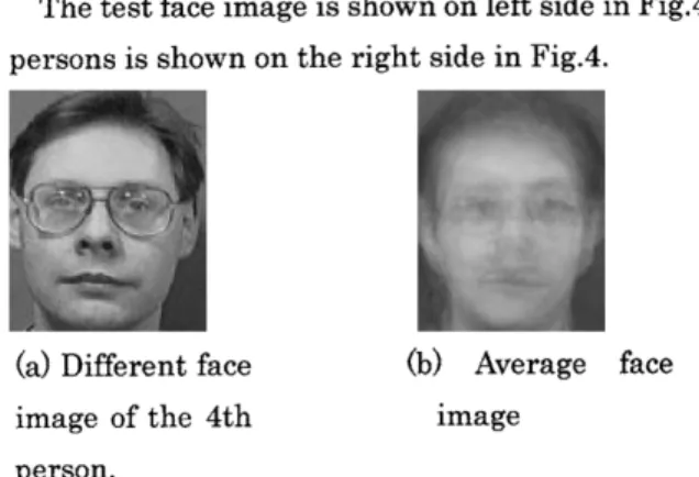
The test face image is shown on left side in Fig.4. Also, the average face image of the 9 persons is shown on the right side in Fig.4.
(a) Different face image of the 4th person.
(b) Average face image
Fig.4 Test face image (left) and average face image.
The values of the L_2 norm, between the vector of the projected test face image (different face image of the 4th person) and the vectors of the projected training face images, are evaluated by the snapshot PCA method and the snapshot QR decomposition method.
3.2.3 Face recognition results (1) Snapshot PCA method
The values of the L_2 norm, calculated by the snapshot PCA method, are shown in Table 3.
Table 3 Values of the L_2 norm by the snapshot PCA method.
(2) Snapshot QR decomposition method
shown in Table 4.
Table 4 Values of the L_2 norm by the snapshot QR decomposition method.
3.2.4 Review of the results
In this section, the recognition experiment is implemented by using 9 human face
images. As a result, it is shown that there are differences in the values of the L_2 norm,
between the vector of the projected test face image and the vectors of the projected
training face images, by the snapshot PCA method, when compared with those by the
snapshot QR decomposition method. From Table 3 and Table 4, Fig.5 is illustrated.
Fig.5 shows that the values of the L_2 norm by the snapshot QR decomposition
method take wider range than those by the snapshot PCA method. The minimum value
of the L_2 norm by the snapshot QR decomposition method for the 4th person is
smaller than that by the snapshot PCA method.
Also, in the case of the snapshot PCA method, the computation time for the face
recognition is 22.3900 seconds, whereas it takes 23.3120 seconds when the snapshot QR
decomposition is used. This shows that the snapshot PCA method is slightly shorter
than the time consumed by the snapshot QR decomposition method.
Fig.5 Values of the L_2 norm, between the vector of the projected test face image and
the vectors of the 9 projected training face images, vs. person No. by the snapshot PCA
method and the snapshot QR decomposition method.
3.3. Face recognition using 40 face images
In this section, the number of the training face images, used for the face recognition, is increased from 9 to 40. The aim of this section is to investigate the differences on the values of the L_2 norms and the computation times between the snapshot QR
decomposition method and the snapshot PCA method.
3.3.1 Face images used in the recognition
Fig.6 Training face images of 40 persons.
3.3.2 Test image and average face image
As a test image, a different face image of the 20th person is used.
(a) Different face image of the
20th person
(b) Average face image of 40 persons
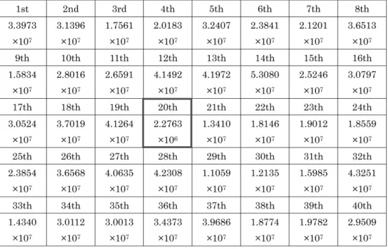
3.3.3 Face recognition results (1) Snapshot PCA method
The values of the L_2 norm calculated by the snapshot PCA method are shown in Table 5.
Table 5 Values of L_2 norm by the snapshot PCA method.
(2) Snapshot QR decomposition method
The values of the L_2 norm calculated by the snapshot QR decomposition method are shown in Table 6.
3.3.4 Review of the results
In this section, the face recognition experiment has been implemented using 40
training face images. From Table 5 and Table 6, Fig.8 is illustrated. Fig.8 shows that
the values of the L_2 norm by the snapshot QR decomposition method take wider
range than those by the snapshot PCA method. The minimum value of the L_2 norm by
the QR decomposition method for the 20th person is smaller than that by the
snapshot PCA.
It is also interesting, in comparison with the case of 9 training face images, to
investigate on the computation time consumed for the case of the 40 training face
images. In the case of snapshot PCA method, the computation time for the face
recognition is 140.9220 seconds, whereas it takes 112.9840 seconds when the snapshot
QR decomposition method is used. Since the computation time by the snapshot QR
decomposition method is fairly shorter than the snapshot PCA method, the snapshot QR
decomposition method is much preferable, in face recognition, to the snapshot PCA
method.
Throughout the simulation, MATLAB program is implemented by the personal
Fig.8 Values of L_2 norm, between the vector of the projected test face image and the
vectors of the 40 projected training face images, vs. person No. by the snapshot PCA
method and snapshot QR decomposition method.
In this paper, the snapshot QR decomposition method is presented. The recognition method is compared with the snapshot PCA method in section 3. As a result, in the case of the simulation for the image with 3 x 3 gray levels, there are no differences on the values of the L_2 norm by the both methods. In contrast, when the human face images are used, the differences appear in the values of the L_2 norm between the two methods. This result might be caused by using the face training images with 256 of pixel levels in contrast to the case of using four simple training images with 3 x 3 gray levels.
In the snapshot PCA method and the snapshot QR decomposition method, the test face image is correctly recognized for the both cases using the 40 training face images and 9 training face images from the minimum values of the L_2 norm between the vector of the projected test image and the vectors of the projected training images.
By the snapshot PCA method with 9 training face images, it takes 22.3900 seconds, which might be compared with 23.3120 seconds by the snapshot QR decomposition method. In the face recognition, the snapshot PCA method is slightly faster than the snapshot QR decomposition method. Meanwhile, the computation times, in the face recognition using the 40 training face images, are 140.9220 seconds by the snapshot PCA method and 112.9840 seconds by the snapshot QR decomposition method. This indicates, in the case of 40 training face images, the computation time by the snapshot QR decomposition method is considerably reduced from that by the snapshot PCA method. The face recognition results are correct and values of the L_2 norm in the snapshot QR decomposition method take the wider range than in the snapshot PCA method. On the basis of these considerations, the snapshot QR decomposition method, proposed in this paper, can be applied more efficiently to the face recognition problem than the snapshot PCA method.
References
[1] Moon. H. and P.J. Phillips (2001), Computational and performance aspects of
PCA-based face recognition algorithms, Perception, 30, 303-321.
[2] Yambor, W. S. (2000), Analysis of PCA-based and Fisher discriminant-based image
recognition algorithms, Computer Science Technical Report, Computer Science
Department, Colorado State University.
QR-decomposition, IEEE Trans. Pattern Analysis and Machine Intelligence, 27, 929-941.
[4] Face image database ORL : Visualizing PCA's perfomance in Face Recognition: http://people.cs.uchicago.edu/~dinaj/vis/or1/
[5] Horn, R. and Johnson, C., Matrix Analysis, New York, Cambridge University Press, 1985.
[6] Trucco, E. and Verri, A., Introductory Techniques for 3-D Computer Vision, New Jeersey, Prentice-Hall, 1988